UMAP on low rank matrix and loadings

Abstract

To understand the disease network, we plot an interactive UMAP from the loadings of the latent factors.

Setup

We have to first load a bunch of useful tools including UMAP and Bokeh.

import os
import numpy as np
import pandas as pd
import pickle
import re

import matplotlib.pyplot as plt
from pymir import mpl_stylesheet
from pymir import mpl_utils

mpl_stylesheet.banskt_presentation(splinecolor = 'black', dpi = 120)

import umap
from bokeh.plotting import figure as bokeh_figure
from bokeh.plotting import show as bokeh_show
from bokeh.layouts import column as bokeh_column
from bokeh.io import output_notebook
from bokeh.models import ColumnDataSource
from bokeh.models import HoverTool
from bokeh.models import CategoricalColorMapper

output_notebook()

Loading BokehJS ...

Load data and results

Here, we explore the low rank model from nuclear norm minimization with the sparse matrix.

data_dir = "/gpfs/commons/home/sbanerjee/work/npd/PanUKB/data"
result_dir = "/gpfs/commons/home/sbanerjee/work/npd/PanUKB/results/nnsparsh"

zscore_df = pd.read_pickle(os.path.join(data_dir, f"modselect/zscore_all.pkl"))
trait_df  = pd.read_pickle(os.path.join(data_dir, f"modselect/traits_all_with_desc.pkl"))
zscore_df_noRx = pd.read_pickle(os.path.join(data_dir, f"modselect/zscore_noRx.pkl"))

method = 'nnm_sparse'

res_filename = os.path.join(result_dir, "full", f"{method}_model.pkl")
with (open(res_filename, "rb")) as fh:
    lowrank_model = pickle.load(fh)
    
res_filename_noRx = os.path.join(result_dir, "noRx", f"{method}_model.pkl")
with (open(res_filename_noRx, "rb")) as fh:
    lowrank_model_noRx = pickle.load(fh)

X = np.array(zscore_df.drop(labels = ['rsid'], axis = 1).values.T)
X_cent = X - np.mean(X, axis = 0, keepdims = True)

X_noRx = np.array(zscore_df_noRx.values.T)
X_noRx_cent = X_noRx - np.mean(X_noRx, axis = 0, keepdims = True)

lowX = lowrank_model['X_']
lowX_cent = lowX - np.mean(lowX, axis = 0, keepdims = True)
lowX_std = lowX_cent / np.sqrt(np.prod(lowX_cent.shape))

lowX_noRx = lowrank_model_noRx['X_']
lowX_noRx_cent = lowX_noRx - np.mean(lowX_noRx, axis = 0, keepdims = True)
lowX_noRx_std = lowX_noRx_cent / np.sqrt(np.prod(lowX_noRx_cent.shape))

print ("Nuclear Norms")
print (f"Low rank model: {np.linalg.norm(lowX, ord = 'nuc'):.3f}")
print (f"Low rank model without Rx: {np.linalg.norm(lowX_noRx, ord = 'nuc'):.3f}")
print (f"Input data: {np.linalg.norm(X, ord = 'nuc'):.3f}")
print (f"Input data (mean centered): {np.linalg.norm(X_cent, ord = 'nuc'):.3f}")

Nuclear Norms
Low rank model: 8050.750
Low rank model without Rx: 8059.143
Input data: 496751.155
Input data (mean centered): 495872.387

Compute loadings

We compute the loadings from the SVD of the low rank approximation of the input data. We use the top 100 factors and their loadings.

To-Do: Save the loadings and factors so that we don’t have to calculate it every time.

def compute_loadings_factors(X, k = None):
    #X_cent = mpy_simulate.do_standardize(X, scale = False)
    #X_cent /= np.sqrt(np.prod(X_cent.shape))
    U, S, Vt = np.linalg.svd(X, full_matrices = False)
    S2 = np.square(S)
    explained_variance = S2 / np.sum(S2)
    if k is None:
        k = np.where(explained_variance < 1e-12)[0][0] - 1
    U_low = U[:, :k]
    S_low = S[:k]
    factors = Vt[:k, :].T
    loadings = U_low @ np.diag(S_low)
    return U_low, S_low, loadings, factors

U0, S0, loadings0, factors0 = compute_loadings_factors(lowX_std)
U1, S1, loadings1, factors1 = compute_loadings_factors(lowX_noRx_std)
U2, S2, loadings2, factors2 = compute_loadings_factors(X_cent)
U3, S3, loadings3, factors3 = compute_loadings_factors(X_noRx_cent)

nnm_loadings  = loadings0.copy()
nnm_loadings_noRx = loadings1.copy()
tsvd_loadings = U2[:, :loadings0.shape[1]] @ np.diag(S2[:loadings0.shape[1]])
tsvd_loadings_noRx = U3[:, :loadings1.shape[1]] @ np.diag(S3[:loadings1.shape[1]])

def make_single_plot_principal_components(ax, i, j, comps, labels, label_color_dict, alphas):
    pc1 = comps[:, j]
    pc2 = comps[:, i]
    for label, color in label_color_dict.items():
        idx = np.where(labels == label)[0]
        if idx.shape[0] > 0:
            ax.scatter(pc1[idx], pc2[idx], s = 50, alpha = alphas[idx], label = label, color = color)
    return

def make_plot_principal_components_diag(pcomp, class_labels, class_colors,
        h2 = None, alpha_factor = 10,
        ncomp = 6,
        subplot_h = 2.0, bgcolor = "#F0F0F0"):

    '''
    pcomp: principal components
    class_labels: the class of each sample
    class_colors: dict of class colors for each label
    '''

    nrow = ncomp - 1
    ncol = ncomp - 1
    figw = ncol * subplot_h + (ncol - 1) * 0.3 + 1.2
    figh = nrow * subplot_h + (nrow - 1) * 0.3 + 1.5

    fig = plt.figure(figsize = (figw, figh))
    axmain = fig.add_subplot(111)
    axs = list()
    
    if h2 is None:
        alpha_arr = np.full([pcomp.shape[0],], 0.6)
    else:
        alpha_arr = np.array([min(0.6, alpha_factor * abs(x)) for x in h2])

    for i in range(1, nrow + 1):
        for j in range(ncol):
            ax = fig.add_subplot(nrow, ncol, ((i - 1) * ncol) + j + 1)

            ax.tick_params(bottom = False, top = False, left = False, right = False,
                labelbottom = False, labeltop = False, labelleft = False, labelright = False)
            if j == 0: ax.set_ylabel(f"PC{i + 1}")
            if i == nrow: ax.set_xlabel(f"PC{j + 1}")
            if i > j:
                ax.patch.set_facecolor(bgcolor)
                ax.patch.set_alpha(0.3)
                make_single_plot_principal_components(ax, i, j, pcomp, class_labels, class_colors, alpha_arr)
                for side, border in ax.spines.items():
                    border.set_color(bgcolor)
            else:
                ax.patch.set_alpha(0.)
                for side, border in ax.spines.items():
                    border.set_visible(False)

            if i == 1 and j == 0:
                mhandles, mlabels = ax.get_legend_handles_labels()
            axs.append(ax)

    axmain.tick_params(bottom = False, top = False, left = False, right = False,
        labelbottom = False, labeltop = False, labelleft = False, labelright = False)
    for side, border in axmain.spines.items():
        border.set_visible(False)
    #axmain.legend(handles = mhandles, labels = mlabels, loc = 'upper right', bbox_to_anchor = (0.9, 0.9))

    plt.tight_layout()
    return axmain, axs


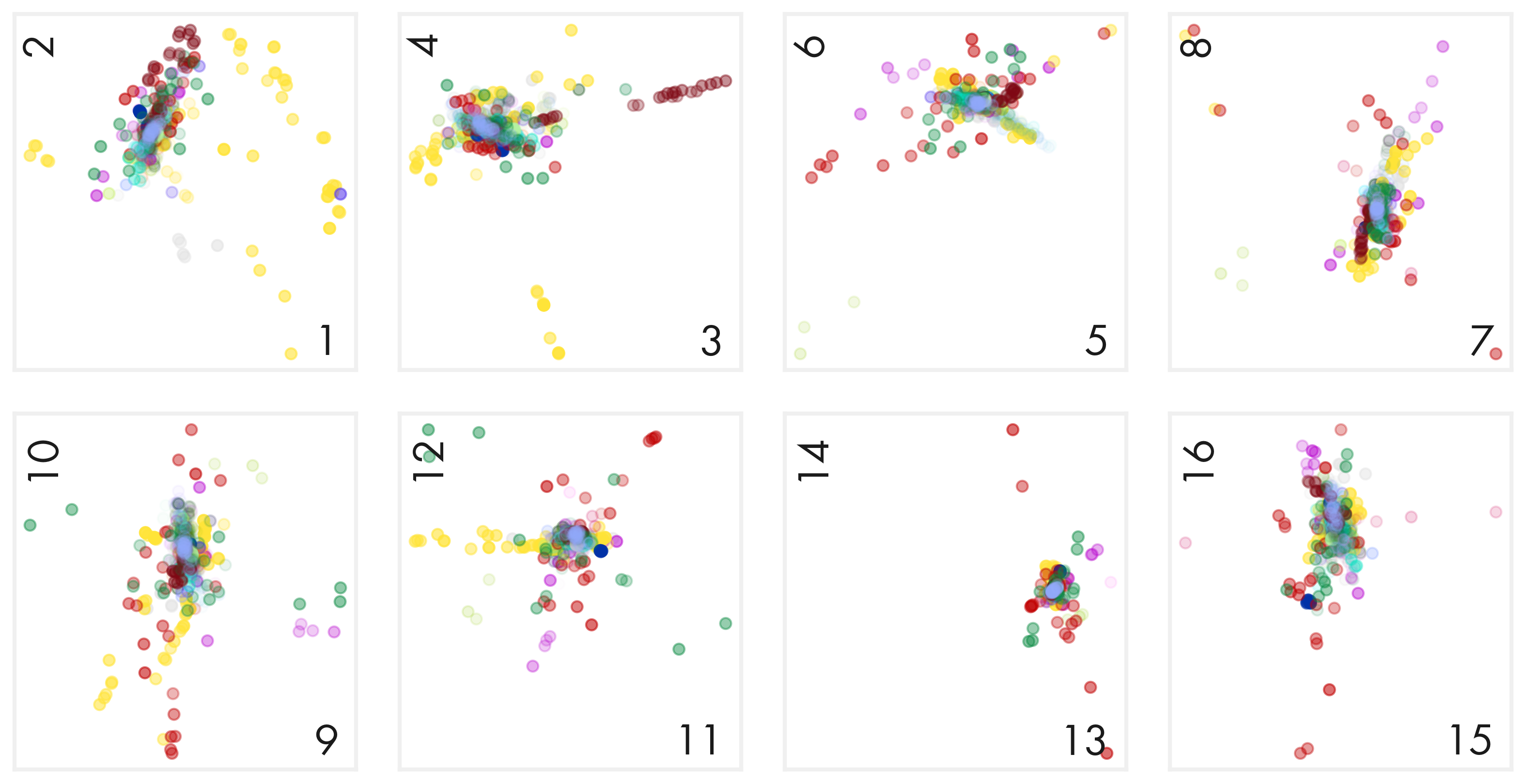
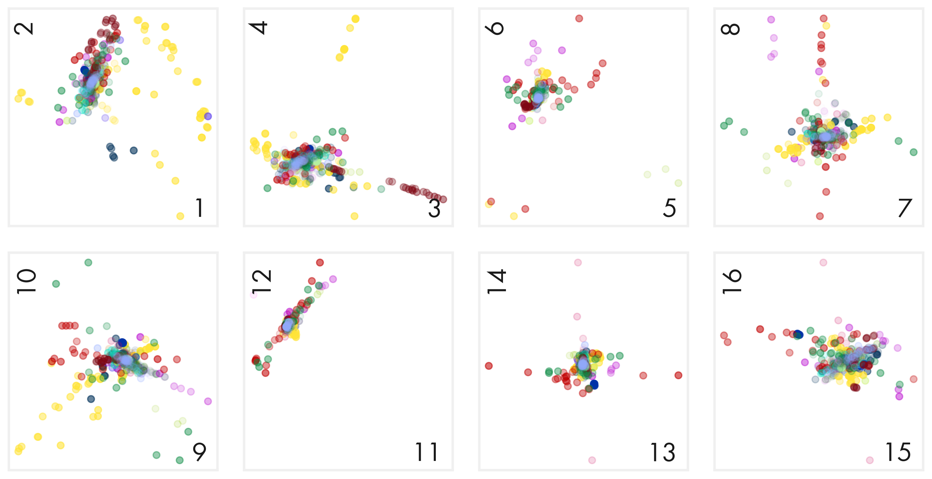
def make_plot_principal_components(pcomp, class_labels, class_colors,
        h2 = None, alpha_factor = 10,
        ncomp = None, ncol = 4,
        subplot_h = 2.0, bgcolor = "#F0F0F0"):

    '''
    pcomp: principal components
    class_labels: the class of each sample
    class_colors: dict of class colors for each label
    '''
    
    if ncomp is None: ncomp = pcomp.shape[1]
    ncomp = int(ncomp / 2) * 2

    nrow = int(np.ceil(ncomp / 2 / ncol)) 
    figw = ncol * subplot_h + (ncol - 1) * 0.3 + 2.0
    figh = nrow * subplot_h + (nrow - 1) * 0.3 + 1.5

    fig = plt.figure(figsize = (figw, figh))
    axmain = fig.add_subplot(111)
    axs = list()
    
    if h2 is None:
        alpha_arr = np.full([pcomp.shape[0],], 0.6)
    else:
        alpha_arr = np.array([min(0.6, alpha_factor * abs(x)) for x in h2])
        
    for i in range(int(ncomp / 2)):
        ix = i * 2
        iy = ix + 1
        ax = fig.add_subplot(nrow, ncol, i + 1)
        
        ax.tick_params(bottom = False, top = False, left = False, right = False,
            labelbottom = False, labeltop = False, labelleft = False, labelright = False)
        ax.set_xlabel(f"{ix + 1}", labelpad = -18, x = 0.95, ha = 'right')
        ax.set_ylabel(f"{iy + 1}", labelpad = -18, y = 0.95, ha = 'right')
        ax.patch.set_facecolor(bgcolor)
        ax.patch.set_alpha(0.3)
        make_single_plot_principal_components(ax, iy, ix, pcomp, class_labels, class_colors, alpha_arr)
        for side, border in ax.spines.items():
            border.set_color(bgcolor)
        axs.append(ax)

    axmain.tick_params(bottom = False, top = False, left = False, right = False,
        labelbottom = False, labeltop = False, labelleft = False, labelright = False)
    for side, border in axmain.spines.items():
        border.set_visible(False)
    #axmain.legend(handles = mhandles, labels = mlabels, loc = 'upper right', bbox_to_anchor = (0.9, 0.9))

    plt.tight_layout()
    return axmain, axs

hex_colors_40 = [
    "#e3e3e30d",
    "#084609",
    "#ff4ff4",
    "#01d94a",
    "#b700ce",
    "#91c900",
    "#5f42ed",
    "#5fa200",
    "#8d6dff",
    "#c9f06b",
    "#0132a7",
    "#ffbb1f",
    "#0080ed",
    "#f56600",
    "#3afaf5",
    "#c10001",
    "#01e698",
    "#a20096",
    "#00e2c1",
    "#ff5ac8",
    "#008143",
    "#cd0057",
    "#4aeeff",
    "#8c001a",
    "#b5f2a2",
    "#5d177d",
    "#a99900",
    "#e299ff",
    "#5b6b00",
    "#96aeff",
    "#a46f00",
    "#007acb",
    "#ff9757",
    "#00a8e0",
    "#ff708e",
    "#baefc7",
    "#622b25",
    "#c8c797",
    "#885162",
    "#ffb7a5",
    "#ffa3c3"]

llm_methods = [
    "ls-da3m0ns/bge_large_medical",
    "medicalai/ClinicalBERT",
    "emilyalsentzer/Bio_ClinicalBERT",
]

llm_ctypes = ["community", "kmeans"]
llm_clusters = {method : { x : None for x in llm_ctypes } for method in llm_methods}
llm_outdir = "/gpfs/commons/home/sbanerjee/work/npd/PanUKB/results/llm"

for method in llm_methods:
    for ctype in llm_ctypes:
        m_filename = os.path.join(llm_outdir, f"{method}/{ctype}_clusters.pkl")
        with open(m_filename, "rb") as fh:
            llm_clusters[method][ctype] = pickle.load(fh)
            
def get_llm_cluster_labels(selectidx, method, ctype):
    clusteridx = np.full([selectidx.shape[0],], -1)
    for i, ccomps in enumerate(llm_clusters[method][ctype]):
        for idx in ccomps:
            clusteridx[idx] = i
    return clusteridx

llm_method   = "ls-da3m0ns/bge_large_medical"
llm_ctype    = "kmeans"
labels       = get_llm_cluster_labels(np.array(trait_df.index), llm_method, llm_ctype)
label_colors = { label : hex_colors_40[i] for i, label in enumerate(np.unique(labels)) }
trait_h2     = trait_df['estimates.final.h2_observed'].fillna(1e-6).tolist()
alpha_factor = 2.0 if llm_ctype == "kmeans" else 2.0

axmain, axs = make_plot_principal_components(nnm_loadings, labels, label_colors, h2 = trait_h2, alpha_factor = alpha_factor)
plt.show()

labels        = get_llm_cluster_labels(np.array(trait_df.index), llm_method, llm_ctype)
trait_df_noRx = trait_df.query('trait_type != "prescriptions"')
labels_noRx   = [labels[i] for i in trait_df_noRx.index]
trait_h2      = trait_df_noRx['estimates.final.h2_observed'].fillna(1e-6).tolist()

axmain, axs = make_plot_principal_components(nnm_loadings_noRx, labels_noRx, label_colors, h2 = trait_h2, alpha_factor = alpha_factor)
plt.show()

Apply UMAP

We apply UMAP on four different data:

1. NNM loadings of all phenotypes
2. tSVD loadings of all phenotypes
3. NNM loadings of all phenotypes except prescriptions.
4. tSVD loadings of all phenotypes except prescriptions.

def get_umap_embedding(loadings, metric = 'cosine', n_neighbors = 15, min_dist = 0.4):
    reducer = umap.UMAP(n_neighbors = n_neighbors, metric = metric, min_dist = min_dist)
    return reducer.fit_transform(loadings)

umap_metrics = ['euclidean', 'cosine']
nnm_embedding       = { m : get_umap_embedding(nnm_loadings, metric = m) for m in umap_metrics }
tsvd_embedding      = { m : get_umap_embedding(tsvd_loadings, metric = m) for m in umap_metrics }
nnm_embedding_noRx  = { m : get_umap_embedding(nnm_loadings_noRx, metric = m) for m in umap_metrics }
tsvd_embedding_noRx = { m : get_umap_embedding(tsvd_loadings_noRx, metric = m) for m in umap_metrics }

Interactive Plots

Each point is a PanUKB phenotype, colored according to the clusters identified by LLM models from the trait descriptions. The opaciy of each point is proportional to the estimated heritability of the trait.

def get_bokeh_plot(embedding, trait_labels, trait_df, plot_title, color_palette = hex_colors_40, alpha_factor = 10):
    
    plot_dict = dict(
        x = embedding[:, 0],
        y = embedding[:, 1],
        trait_type_code = [f"{x}" for x in trait_labels],
        h2_fill_alpha = [min(0.6, alpha_factor * x) for x in trait_df['estimates.final.h2_observed'].fillna(1e-6).tolist()],
        h2_line_alpha = [min(0.8, 1.3 * alpha_factor * x) for x in trait_df['estimates.final.h2_observed'].fillna(1e-6).tolist()],
        fulldesc = [f"{i} | {trait_df.loc[i, 'short_description']} | {trait_df.loc[i, 'estimates.final.h2_observed']:.3f} | {trait_df.loc[i, 'Neff']:.2f}" 
                    for i in trait_df.index],
    )

    color_mapping = CategoricalColorMapper(factors = [f"{x}" for x in np.unique(trait_labels)], palette = color_palette)

    plot_tooltips = [
        ("Desc", "@fulldesc"),
    ]

    ax = bokeh_figure(
        width = 800, height = 800, 
        tooltips = plot_tooltips,
        title = plot_title,
    )

    ax.circle('x', 'y', size = 10, 
        source = ColumnDataSource(plot_dict), 
        color = dict(field='trait_type_code', transform = color_mapping),
        line_alpha = dict(field='h2_line_alpha'),
        fill_alpha = dict(field='h2_fill_alpha'),
    )
    ax.title.text_font_size = '16pt'
    ax.title.text_font_style = 'normal'
    ax.title.text_font = 'tahoma'
    ax.axis.major_label_text_font_size = '20pt'
    ax.axis.axis_line_width = 2
    ax.axis.major_tick_line_width = 2
    ax.grid.visible = False
    return ax

bokeh_colors = hex_colors_40.copy()
bokeh_colors[0] = "#3c3c3c0d"
llm_method   = "ls-da3m0ns/bge_large_medical"
llm_ctype    = "community"
alpha_factor = 10 if llm_ctype == "kmeans" else 100
labels       = get_llm_cluster_labels(np.array(trait_df.index), llm_method, llm_ctype)

axlist = list()
for metric in umap_metrics:
    ax = get_bokeh_plot(
        nnm_embedding[metric], labels, trait_df, 
        f"NNM, {metric}, {llm_method}, {llm_ctype} clustering",
        alpha_factor = alpha_factor,
        color_palette = bokeh_colors
    )
    axlist.append(ax)
    
# put all the plots in a VBox
p = bokeh_column(*axlist)

# show the results
bokeh_show(p)

(a) UMAP embeddings of the NNM loadings.

(b)

Figure 1

axlist = list()
for metric in umap_metrics:
    ax = get_bokeh_plot(
        tsvd_embedding[metric], labels, trait_df, 
        f"tSVD, {metric}, {llm_method}, {llm_ctype} clustering",
        alpha_factor = alpha_factor,
        color_palette = bokeh_colors
    )
    axlist.append(ax)
    
# put all the plots in a VBox
p = bokeh_column(*axlist)

# show the results
bokeh_show(p)

(a) UMAP embeddings of the tSVD embeddings.

(b)

Figure 2

labels        = get_llm_cluster_labels(np.array(trait_df.index), llm_method, llm_ctype)
trait_df_noRx = trait_df.query('trait_type != "prescriptions"')
labels_noRx   = [labels[i] for i in trait_df_noRx.index]

axlist = list()
for metric in umap_metrics:
    ax = get_bokeh_plot(
        nnm_embedding_noRx[metric], labels_noRx, trait_df_noRx, 
        f"NNM, {metric}, {llm_method}, {llm_ctype} clustering",
        alpha_factor = alpha_factor,
        color_palette = bokeh_colors
    )
    axlist.append(ax)
    
# put all the plots in a VBox
p = bokeh_column(*axlist)

# show the results
bokeh_show(p)

(a) UMAP embeddings of the NNM loadings except prescriptions.

(b)

Figure 3

axlist = list()
for metric in umap_metrics:
    ax = get_bokeh_plot(
        tsvd_embedding_noRx[metric], labels_noRx, trait_df_noRx, 
        f"tSVD, {metric}, {llm_method}, {llm_ctype} clustering",
        alpha_factor = alpha_factor,
        color_palette = bokeh_colors
    )
    axlist.append(ax)
    
# put all the plots in a VBox
p = bokeh_column(*axlist)

# show the results
bokeh_show(p)

(a) UMAP embeddings of the tSVD loadings except prescriptions.

(b)

Figure 4