Understanding the biology of diseases

Abstract

We attempt to characterize the biology of diseases from the low dimensional representation of the PanUKB summary statistics.

import os
import re
import numpy as np
import pandas as pd
import pickle

import matplotlib.pyplot as plt
from adjustText import adjust_text
import textalloc
import umap

from scipy.cluster import hierarchy as sp_hierarchy
from scipy.spatial import procrustes as sp_procrustes

from pymir import mpl_stylesheet
from pymir import mpl_utils
mpl_stylesheet.banskt_presentation(splinecolor = 'black', dpi = 120, colors = 'kelly')
from matplotlib.gridspec import GridSpec

import sys
sys.path.append("../utils/")
import simulate as mpy_simulate
import plot_functions as mpy_plotfn

from bokeh.plotting import figure as bokeh_figure
from bokeh.plotting import show as bokeh_show
from bokeh.io import output_notebook
from bokeh.models import ColumnDataSource

output_notebook()

Loading BokehJS ...

source = ColumnDataSource(data=dict(
    x=[1, 2, 3, 4, 5],
    y=[2, 5, 8, 2, 7],
    desc=['A', 'b', 'C', 'd', 'E'],
))

TOOLTIPS = [
    ("index", "$index"),
    ("(x,y)", "($x, $y)"),
    ("desc", "@desc"),
]

p = bokeh_figure(width=400, height=400, tooltips=TOOLTIPS,
           title="Mouse over the dots")

p.scatter('x', 'y', size=20, source=source)

bokeh_show(p)

data_dir = "/gpfs/commons/home/sbanerjee/work/npd/PanUKB/data"
result_dir = "/gpfs/commons/home/sbanerjee/work/npd/PanUKB/results/nnsparsh/full/"

zscore_df = pd.read_pickle(os.path.join(data_dir, f"modselect/zscore_all.pkl"))
trait_df  = pd.read_pickle(os.path.join(data_dir, f"modselect/traits_all.pkl"))

variant_filename = f"{data_dir}/allvar.pruned.closesttss.hugo"
variant_df       = pd.read_csv(variant_filename, sep = '\t')

method = 'nnm_sparse'

res_filename = os.path.join(result_dir, f"{method}_model.pkl")
with (open(res_filename, "rb")) as fh:
    lowrank_model = pickle.load(fh)

lowrank_model.keys()

dict_keys(['max_iter_', 'model_', 'svd_method_', 'svd_max_iter_', 'simplex_method_', 'stop_criteria_', 'tol_', 'step_size_tol_', 'fxrel_tol_', 'show_progress_', 'prog_step_skip_', 'is_debug_', 'suppress_warnings_', 'is_benchmark_', 'benchmark_method_', 'weight_', 'mask_', 'weight_mask_', 'Y_', 'rank_', 'l1_thres_', 'fm_list_', 'fl_list_', 'fx_list_', 'dg_list_', 'st_list_', 'cpu_time_', 'convergence_msg_', 'X_', 'M_'])

X = np.array(zscore_df.drop(labels = ['rsid'], axis = 1).values.T)
X_cent = X - np.mean(X, axis = 0, keepdims = True)
lowX = lowrank_model['X_']
lowX_cent = lowX - np.mean(lowX, axis = 0, keepdims = True)
lowX_std = lowX_cent / np.sqrt(np.prod(lowX_cent.shape))

print ("Nuclear Norms")
print (f"Low rank model: {np.linalg.norm(lowX, ord = 'nuc'):.3f}")
print (f"Input data: {np.linalg.norm(X, ord = 'nuc'):.3f}")
print (f"Input data (mean centered): {np.linalg.norm(X_cent, ord = 'nuc'):.3f}")

Nuclear Norms
Low rank model: 8050.750
Input data: 496751.155
Input data (mean centered): 495872.387

# o1 = sp_hierarchy.leaves_list(sp_hierarchy.linkage(np.cov(X_cent), method = 'centroid'))
# o2 = sp_hierarchy.leaves_list(sp_hierarchy.linkage(np.cov(lowX_std), method = 'centroid'))

fig = plt.figure(figsize = (18, 8))
ax1 = fig.add_subplot(121)
ax2 = fig.add_subplot(122)

mpy_plotfn.plot_covariance_heatmap(ax1, X_cent[o1, :], vmax = 0.1)
mpy_plotfn.plot_covariance_heatmap(ax2, lowX_cent[o2, :], vmax = 0.05)

ax1.set_title("Input data", pad = 20)
ax2.set_title("Low-dimensional data", pad = 20)
plt.tight_layout(w_pad = 4.0)
plt.show()

def compute_loadings_factors(X, k = None):
    #X_cent = mpy_simulate.do_standardize(X, scale = False)
    #X_cent /= np.sqrt(np.prod(X_cent.shape))
    U, S, Vt = np.linalg.svd(X, full_matrices = False)
    S2 = np.square(S)
    explained_variance = S2 / np.sum(S2)
    if k is None:
        k = np.where(explained_variance < 1e-12)[0][0] - 1
    U_low = U[:, :k]
    S_low = S[:k]
    factors = Vt[:k, :].T
    loadings = U_low @ np.diag(S_low)
    return U_low, S_low, loadings, factors

U0, S0, loadings0, factors0 = compute_loadings_factors(lowX)
U1, S1, loadings1, factors1 = compute_loadings_factors(lowX_std)
U2, S2, loadings2, factors2 = compute_loadings_factors(X_cent)

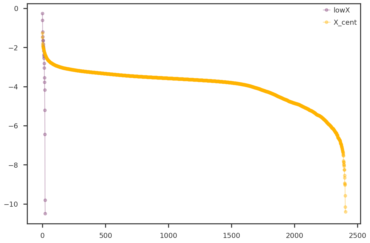
fig = plt.figure(figsize = (12, 8))
ax1 = fig.add_subplot(111)
ax1.plot(np.arange(S0.shape[0]), np.log10(np.square(S0) / np.sum(np.square(S0))), marker = 'o', label = 'lowX', alpha = 0.4)
#ax1.plot(np.arange(S1.shape[0]), np.log10(np.square(S1) / np.sum(np.square(S1))), marker = 'o', label = 'lowX_std', alpha = 0.4)
ax1.plot(np.arange(S2.shape[0]), np.log10(np.square(S2) / np.sum(np.square(S2))), marker = 'o', label = 'X_cent', alpha = 0.4)
ax1.legend()
plt.show()

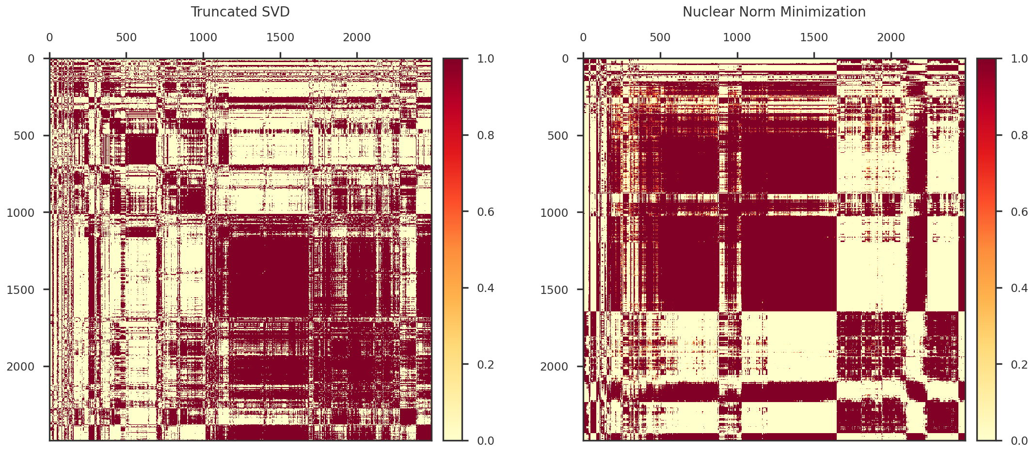
nnm_loadings  = loadings0.copy()
tsvd_loadings = U2[:, :loadings0.shape[1]] @ np.diag(S2[:loadings0.shape[1]])

o1 = sp_hierarchy.leaves_list(sp_hierarchy.linkage(np.cov(tsvd_loadings), method = 'centroid'))
o2 = sp_hierarchy.leaves_list(sp_hierarchy.linkage(np.cov(nnm_loadings), method = 'centroid'))

fig = plt.figure(figsize = (18, 8))
ax1 = fig.add_subplot(121)
ax2 = fig.add_subplot(122)

mpy_plotfn.plot_covariance_heatmap(ax1, tsvd_loadings[o1, :])
mpy_plotfn.plot_covariance_heatmap(ax2, nnm_loadings[o2, :])

ax1.set_title("Truncated SVD", pad = 20)
ax2.set_title("Nuclear Norm Minimization", pad = 20)
plt.tight_layout(w_pad = 4.0)
plt.show()

no_prescription_idx = trait_df[trait_df['trait_type'] != 'prescriptions'].index
nnm_loadings_noprescription  = nnm_loadings[no_prescription_idx, :]
tsvd_loadings_noprescription = tsvd_loadings[no_prescription_idx, :]

import umap
nnm_reducer = umap.UMAP(
    n_neighbors = 10, metric = 'cosine', min_dist = 0.4,
)
nnm_embedding = nnm_reducer.fit_transform(nnm_loadings_noprescription)

tsvd_reducer = umap.UMAP(
    n_neighbors = 10, metric = 'cosine', min_dist = 0.4,
)
tsvd_embedding = tsvd_reducer.fit_transform(tsvd_loadings_noprescription)

trait_type_dict = {
    trait: color for trait, color in zip(
        trait_df['trait_type'].unique().tolist(), 
        mpl_stylesheet.banskt_colors()[:len(trait_df['trait_type'].unique())])
    }

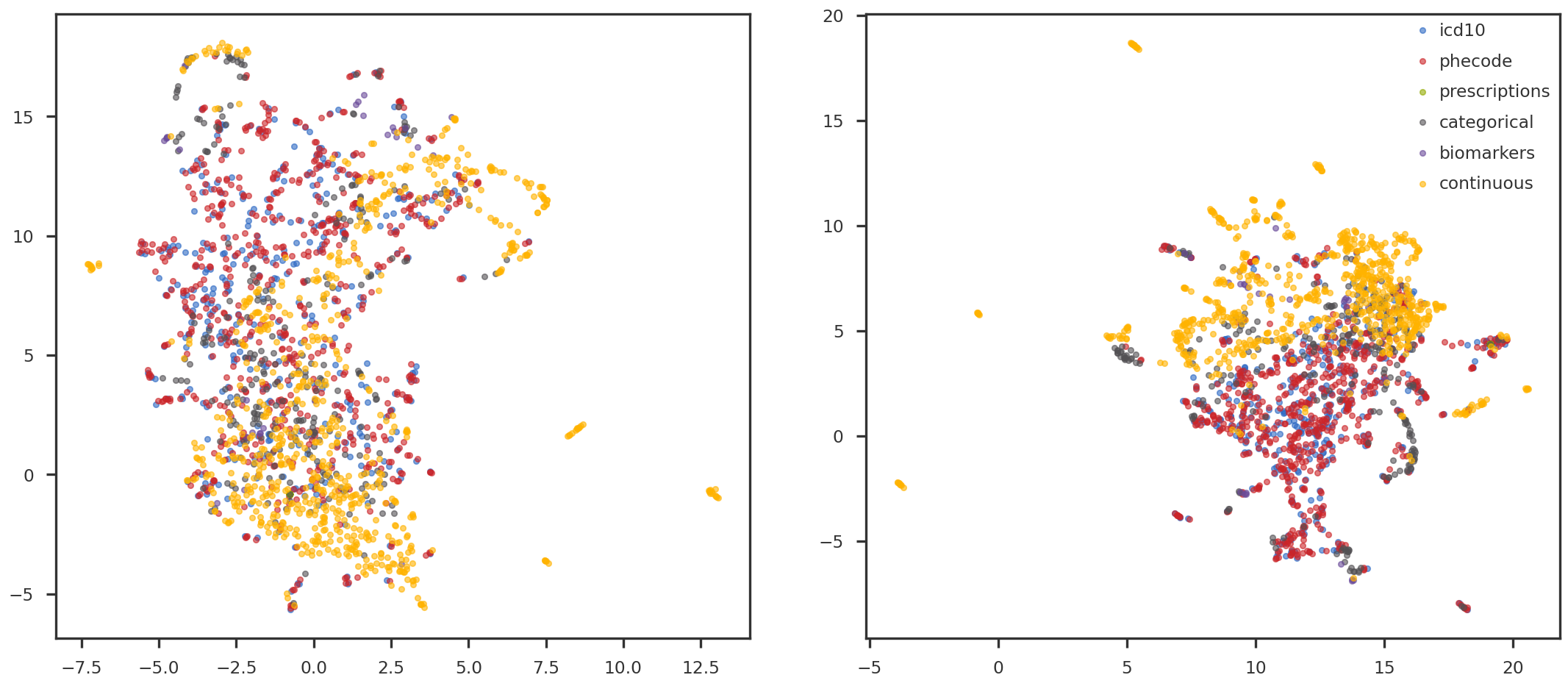
nnm_reducer = umap.UMAP(
    n_neighbors = 10, metric = 'cosine', min_dist = 0.4,
    set_op_mix_ratio = 0.3,
    #densmap=True, dens_lambda=1.0,
    #random_state = 42,
    target_n_neighbors = 50,
)
nnm_embedding = nnm_reducer.fit_transform(nnm_loadings_noprescription)

fig = plt.figure(figsize = (18, 8))
ax1 = fig.add_subplot(121)
ax2 = fig.add_subplot(122)

ipc1 = 4
ipc2 = 5

for trait, color in trait_type_dict.items():
    selectidx = np.array(trait_df[trait_df['trait_type'] == trait].index)
    tidx = np.searchsorted(no_prescription_idx, selectidx)
    ax1.scatter(nnm_embedding[tidx, 0], nnm_embedding[tidx, 1], s = 20, alpha = 0.6, color = color, label = trait)
    ax2.scatter(tsvd_embedding[tidx, 0], tsvd_embedding[tidx, 1], s = 20, alpha = 0.6, color = color, label = trait)
    #ax2.scatter(nnm_loadings_noprescription[tidx, ipc1], nnm_loadings_noprescription[tidx, ipc2], s = 20, alpha = 0.6, color = color, label = trait)

ax2.legend()
plt.tight_layout(w_pad = 4.0)
plt.show()

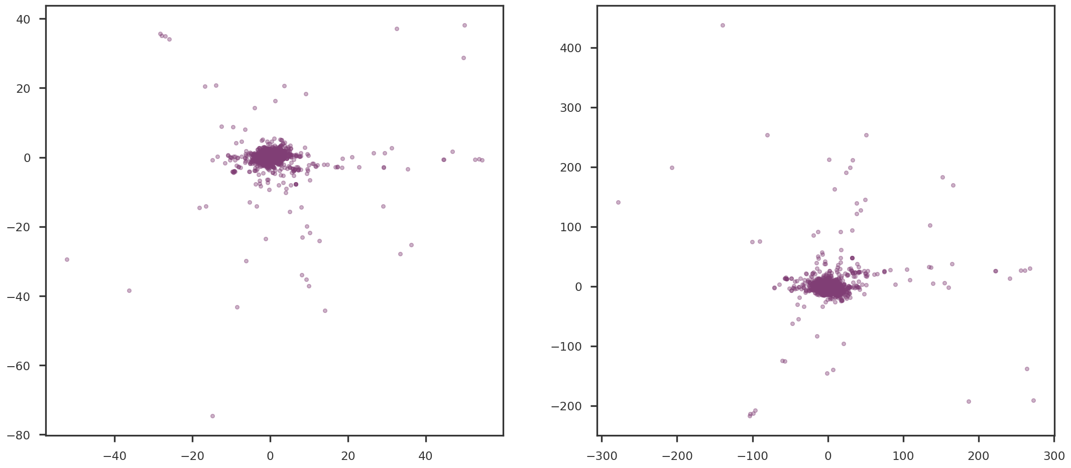
fig = plt.figure(figsize = (18, 8))
ax1 = fig.add_subplot(121)
ax2 = fig.add_subplot(122)

ipc1 = 10
ipc2 = 11

ax1.scatter(loadings0[:, ipc1], loadings0[:, ipc2], s = 20, alpha = 0.4)
ax2.scatter(loadings2[:, ipc1], loadings2[:, ipc2], s = 20, alpha = 0.4)

plt.tight_layout(w_pad = 4.0)
plt.show()

def compute_cos(xmat):
    xmat2 = xmat ** 2
    return xmat2 / np.sum(xmat2, axis = 1, keepdims = True)

def compute_contribution(xmat):
    xmat2 = xmat ** 2
    return xmat2 / np.sum(xmat2, axis = 0, keepdims = True)

U, S, loadings, factors = get_principal_components(lowrank_model['X_'])
cos2_pheno   = compute_cos(loadings)
cos2_variant = compute_cos(factors @ np.diag(S))
contribution_pheno   = compute_contribution(loadings)
contribution_variant = compute_contribution(factors @ np.diag(S))
# cos2_pheno = get_cos2_scores(loadings)
# contribution_pheno = get_contribution_scores(loadings)

List of phenotypes

trait_df['description'].to_list()

['Non-cancer illness code, self-reported',
 'Albumin',
 'Alkaline phosphatase',
 'Alanine aminotransferase',
 'Apolipoprotein A',
 'Apolipoprotein B',
 'Aspartate aminotransferase',
 'Urea',
 'Calcium',
 'Cholesterol',
 'Creatinine',
 'C-reactive protein',
 'Cystatin C',
 'Gamma glutamyltransferase',
 'Glycated haemoglobin (HbA1c)',
 'HDL cholesterol',
 'IGF-1',
 'Phosphate',
 'SHBG',
 'Total protein',
 'Triglycerides',
 'Urate',
 'Pulse rate, automated reading',
 'Time spent watching television (TV)',
 'Morning/evening person (chronotype)',
 'Ventricular rate',
 'P duration',
 'QRS duration',
 'Comparative body size at age 10',
 'Comparative height size at age 10',
 'Sitting height',
 'Fluid intelligence score',
 'Birth weight',
 'Neuroticism score',
 'Forced expiratory volume in 1-second (FEV1), Best measure',
 'Forced vital capacity (FVC), Best measure',
 'Forced expiratory volume in 1-second (FEV1), predicted',
 'Forced expiratory volume in 1-second (FEV1), predicted percentage',
 'Body mass index (BMI)',
 'Weight',
 'Age first had sexual intercourse',
 'Overall health rating',
 'Age hayfever or allergic rhinitis diagnosed by doctor',
 'Age asthma diagnosed by doctor',
 'Posterior thigh lean muscle volume (right)',
 'Posterior thigh lean muscle volume (left)',
 'Visceral adipose tissue volume (VAT)',
 'Abdominal subcutaneous adipose tissue volume (ASAT)',
 'Total trunk fat volume',
 'Year ended full time education',
 'Minimum carotid IMT (intima-medial thickness) at 120 degrees',
 'Mean carotid IMT (intima-medial thickness) at 120 degrees',
 'Maximum carotid IMT (intima-medial thickness) at 120 degrees',
 'Minimum carotid IMT (intima-medial thickness) at 150 degrees',
 'Mean carotid IMT (intima-medial thickness) at 150 degrees',
 'Maximum carotid IMT (intima-medial thickness) at 150 degrees',
 'Minimum carotid IMT (intima-medial thickness) at 210 degrees',
 'Mean carotid IMT (intima-medial thickness) at 210 degrees',
 'Maximum carotid IMT (intima-medial thickness) at 210 degrees',
 'Minimum carotid IMT (intima-medial thickness) at 240 degrees',
 'Mean carotid IMT (intima-medial thickness) at 240 degrees',
 'Maximum carotid IMT (intima-medial thickness) at 240 degrees',
 'Weight',
 'Body fat percentage',
 'Whole body fat mass',
 'Whole body fat-free mass',
 'Whole body water mass',
 'Body mass index (BMI)',
 'Basal metabolic rate',
 'Impedance of whole body',
 'Impedance of leg (right)',
 'Impedance of leg (left)',
 'Impedance of arm (right)',
 'Impedance of arm (left)',
 'Leg fat percentage (right)',
 'Leg fat mass (right)',
 'Leg fat-free mass (right)',
 'Leg predicted mass (right)',
 'Leg fat percentage (left)',
 'Leg fat mass (left)',
 'Leg fat-free mass (left)',
 'Leg predicted mass (left)',
 'Arm fat percentage (right)',
 'Arm fat mass (right)',
 'Arm fat-free mass (right)',
 'Arm predicted mass (right)',
 'Arm fat percentage (left)',
 'Arm fat mass (left)',
 'Arm fat-free mass (left)',
 'Arm predicted mass (left)',
 'Trunk fat percentage',
 'Trunk fat mass',
 'Trunk fat-free mass',
 'Trunk predicted mass',
 'Relative age of first facial hair',
 'Age when periods started (menarche)',
 'Birth weight of first child',
 'Age at first live birth',
 'Age at hysterectomy',
 'Number of cigarettes previously smoked daily',
 'White blood cell (leukocyte) count',
 'Red blood cell (erythrocyte) count',
 'Haemoglobin concentration',
 'Haematocrit percentage',
 'Mean corpuscular volume',
 'Mean corpuscular haemoglobin',
 'Red blood cell (erythrocyte) distribution width',
 'Platelet count',
 'Platelet crit',
 'Mean platelet (thrombocyte) volume',
 'Platelet distribution width',
 'Lymphocyte count',
 'Monocyte count',
 'Neutrophill count',
 'Eosinophill count',
 'Lymphocyte percentage',
 'Monocyte percentage',
 'Neutrophill percentage',
 'Eosinophill percentage',
 'Reticulocyte percentage',
 'Reticulocyte count',
 'Mean reticulocyte volume',
 'Mean sphered cell volume',
 'Immature reticulocyte fraction',
 'High light scatter reticulocyte percentage',
 'High light scatter reticulocyte count',
 'Forced vital capacity (FVC)',
 'Forced expiratory volume in 1-second (FEV1)',
 'Peak expiratory flow (PEF)',
 'Ankle spacing width',
 'Heel Broadband ultrasound attenuation, direct entry',
 'Heel quantitative ultrasound index (QUI), direct entry',
 'Heel bone mineral density (BMD)',
 'Weight, manual entry',
 'Age at menopause (last menstrual period)',
 'Age asthma diagnosed',
 'Age emphysema/chronic bronchitis diagnosed',
 'Age deep-vein thrombosis (DVT, blood clot in leg) diagnosed',
 'Diastolic blood pressure, automated reading',
 'Systolic blood pressure, automated reading',
 'Ankle spacing width (left)',
 'Heel broadband ultrasound attenuation (left)',
 'Heel quantitative ultrasound index (QUI), direct entry (left)',
 'Heel bone mineral density (BMD) (left)',
 'Heel bone mineral density (BMD) T-score, automated (left)',
 'Ankle spacing width (right)',
 'Heel broadband ultrasound attenuation (right)',
 'Heel quantitative ultrasound index (QUI), direct entry (right)',
 'Heel bone mineral density (BMD) (right)',
 'Heel bone mineral density (BMD) T-score, automated (right)',
 'Pulse rate',
 'Round of numeric memory test',
 'Maximum digits remembered correctly',
 'Number of rounds of numeric memory test performed',
 'Duration screen displayed',
 'Hand grip strength (left)',
 'Hand grip strength (right)',
 'Waist circumference',
 'Hip circumference',
 'Standing height',
 'Spherical power (right)',
 'Spherical power (left)',
 '3mm weak meridian (left)',
 '6mm weak meridian (left)',
 '6mm weak meridian (right)',
 '3mm weak meridian (right)',
 'Seated height',
 '6mm asymmetry angle (left)',
 '3mm strong meridian (right)',
 '6mm strong meridian (right)',
 '6mm strong meridian (left)',
 '3mm strong meridian (left)',
 '6mm asymmetry index (left)',
 '6mm asymmetry index (right)',
 'Intra-ocular pressure, corneal-compensated (right)',
 'Intra-ocular pressure, Goldmann-correlated (right)',
 'Corneal hysteresis (right)',
 'Corneal resistance factor (right)',
 'Intra-ocular pressure, corneal-compensated (left)',
 'Intra-ocular pressure, Goldmann-correlated (left)',
 'Corneal hysteresis (left)',
 'Corneal resistance factor (left)',
 'Heel bone mineral density (BMD) T-score, automated',
 'Age completed full time education',
 'Systolic blood pressure, manual reading',
 'Diastolic blood pressure, manual reading',
 'Pulse rate (during blood-pressure measurement)',
 'Albumin/Globulin ratio',
 'Diastolic blood pressure, automated reading, adjusted by medication',
 'Diastolic blood pressure, combined automated + manual reading',
 'Diastolic blood pressure, combined automated + manual reading, adjusted by medication',
 'Diastolic blood pressure, manual reading, adjusted by medication',
 'FEV1/FVC ratio',
 'LDL direct, adjusted by medication',
 'Mean arterial pressure, automated reading',
 'Mean arterial pressure, automated reading, adjusted by medication',
 'Mean arterial pressure, combined automated + manual reading',
 'Mean arterial pressure, combined automated + manual reading, adjusted by medication',
 'Mean arterial pressure, manual reading',
 'Mean arterial pressure, manual reading, adjusted by medication',
 'Non-albumin protein',
 'Pulse pressure, automated reading',
 'Pulse pressure, automated reading, adjusted by medication',
 'Pulse pressure, combined automated + manual reading',
 'Pulse pressure, combined automated + manual reading, adjusted by medication',
 'Pulse pressure, manual reading',
 'Pulse pressure, manual reading, adjusted by medication',
 'Systolic blood pressure, automated reading, adjusted by medication',
 'Systolic blood pressure, combined automated + manual reading',
 'Systolic blood pressure, combined automated + manual reading, adjusted by medication',
 'Systolic blood pressure, manual reading, adjusted by medication',
 'Smoking status, ever vs never',
 'Estimated glomerular filtration rate, serum creatinine',
 'Estimated glomerular filtration rate, cystain C',
 'Estimated glomerular filtration rate, serum creatinine + cystain C',
 'pheno 48 / pheno 49']

trait_df.query("description == 'Body mass index (BMI)'")
# trait_df.query("description == 'Triglycerides'")
# trait_df.query("description == 'Systolic blood pressure, combined automated + manual reading, adjusted by medication'")

	zindex	trait_type	phenocode	pheno_sex	description	description_more	category	BIN_QT	n_cases_EUR	n_controls_EUR	N	Neff	estimates.final.h2_observed
2084	2085	continuous	21001	both_sexes	Body mass index (BMI)	BMI value here is constructed from height and ...	UK Biobank Assessment Centre > Physical measur...	QT	419163	NaN	419163	419163.0	0.262
2144	2145	continuous	23104	both_sexes	Body mass index (BMI)	Body composition estimation by impedance measu...	UK Biobank Assessment Centre > Physical measur...	QT	413186	NaN	413186	413186.0	0.268

zindex = 2085
trait_df.loc[[zindex - 1]]

	zindex	trait_type	phenocode	pheno_sex	description	description_more	category	BIN_QT	n_cases_EUR	n_controls_EUR	N	Neff	estimates.final.h2_observed
2084	2085	continuous	21001	both_sexes	Body mass index (BMI)	BMI value here is constructed from height and ...	UK Biobank Assessment Centre > Physical measur...	QT	419163	NaN	419163	419163.0	0.262

trait_indices = np.array(trait_df.index)
tidx = np.searchsorted(trait_indices, zindex - 1)

top_factor = np.argsort(cos2_pheno[tidx,:])[::-1][0]
top_factor_score = cos2_pheno[tidx, top_factor]
top_traits_idx = np.argsort(contribution_pheno[:,top_factor])[::-1]
top_traits_name = trait_df.loc[trait_indices[top_traits_idx]]['description'].to_list()
top_traits_score = contribution_pheno[top_traits_idx, top_factor]

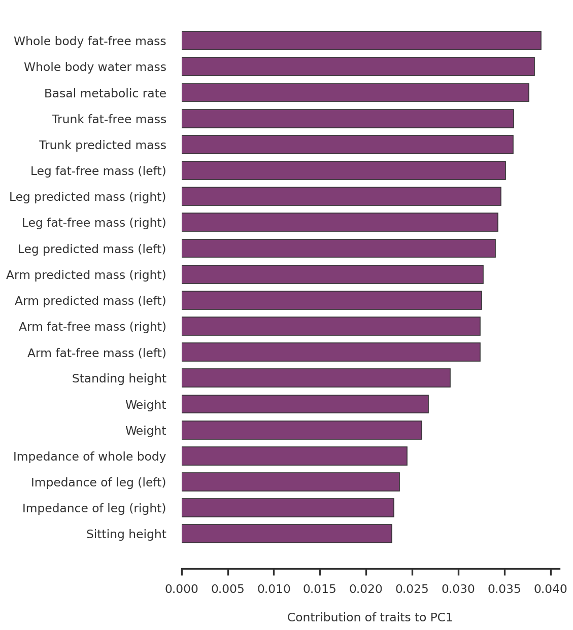
Contribution of traits to factors

def compute_cos(xmat):
    xstd  = xmat / np.sqrt(np.var(xmat, axis = 1, keepdims = True))
    xstd2 = xstd ** 2
    return xstd2 / np.sum(xstd2, axis = 1, keepdims = True)

def compute_contribution(xmat):
    xstd  = xmat / np.sqrt(np.var(xmat, axis = 0, keepdims = True))
    xstd2 = xstd ** 2
    return xstd2 / np.sum(xstd2, axis = 0, keepdims = True)

def compute_contribution(factor):
    return (factor ** 2) / (np.sum(factor ** 2, axis = 0).reshape((1, factor.shape[1])))

def compute_cos(factor):
    return (factor ** 2) / (np.sum(factor ** 2, axis = 1).reshape((factor.shape[0], 1)))

# cos2_pheno         = compute_cos(loadings)
# contribution_pheno = compute_contribution(loadings)
cos2_pheno         = get_cos2_scores(loadings)
contribution_pheno = get_contribution_scores(loadings)

zindex = 2085
trait_indices = np.array(trait_df.index)
tidx = np.searchsorted(trait_indices, zindex - 1)

top_factor = np.argsort(cos2_pheno[tidx,:])[::-1][0]
top_traits_idx = np.argsort(contribution_pheno[:,top_factor])[::-1]
top_traits_name = trait_df.loc[trait_indices[top_traits_idx]]['description'].to_list()
top_traits_score = contribution_pheno[top_traits_idx, top_factor]

fig = plt.figure(figsize = (8, 12))
ax1 = fig.add_subplot(111)

n_plot_traits = 20
xvals = top_traits_score[:n_plot_traits]
yvals = np.arange(n_plot_traits)[::-1]

ax1.barh(yvals, xvals, align = 'center', height = 0.7)
ax1.set_yticks(yvals)
ax1.set_yticklabels(top_traits_name[:n_plot_traits])

for side in ['top', 'right', 'left']:
    ax1.spines[side].set_visible(False)
    
ax1.tick_params(left=False)
ax1.set_xlabel(f"Contribution of traits to PC{top_factor + 1}")

plt.show()

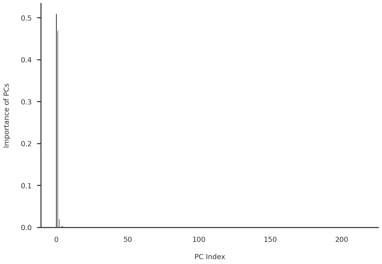
Importance of components

fig = plt.figure(figsize = (12, 8))
ax1 = fig.add_subplot(111)

xvals = np.arange(cos2_pheno.shape[0])
yvals = cos2_pheno[tidx,:]
ax1.bar(xvals, yvals, align = 'center', width = 0.1)

for side in ['top', 'right']:
    ax1.spines[side].set_visible(False)
    
ax1.tick_params(bottom=False)
ax1.set_ylabel(f"Importance of PCs")
ax1.set_xlabel(f"PC Index")

plt.show()

top_factor_dict = {i : list() for i in range(cos2_pheno.shape[0])}
for i, trait_name in enumerate(trait_df['description'].to_list()):
    top_factor = np.argsort(cos2_pheno[i, :])[::-1][0]
    top_factor_dict[top_factor].append(trait_name)

top_factor = 0
top_traits_idx = np.argsort(contribution_pheno[:,top_factor])[::-1]
top_traits_name = trait_df.loc[trait_indices[top_traits_idx]]['description'].to_list()
top_traits_score = contribution_pheno[top_traits_idx, top_factor]

# print (top_factor_dict[top_factor])

fig = plt.figure(figsize = (8, 12))
ax1 = fig.add_subplot(111)

n_plot_traits = 20
xvals = top_traits_score[:n_plot_traits]
yvals = np.arange(n_plot_traits)[::-1]

ax1.barh(yvals, xvals, align = 'center', height = 0.7)
ax1.set_yticks(yvals)
ax1.set_yticklabels(top_traits_name[:n_plot_traits])

for side in ['top', 'right', 'left']:
    ax1.spines[side].set_visible(False)
    
ax1.tick_params(left=False)
ax1.set_xlabel(f"Contribution of traits to PC{top_factor + 1}")

plt.show()

Which variants are contributing to the top factor?

np.square(eigenvals)[3]

0.011598380845155945

tidx

38

cos2_scores_ = compute_cos(pcomps)

np.sum(cos2_scores_[tidx, :])

0.9999999999999998

np.argsort(cos2_scores_[:, tidx])

array([127,  34,  49, 120, 162,  26,  33, 214,  42, 213, 111,  37, 191,
        12, 109, 137, 128, 215, 167,  69,  92, 113, 112,  63, 193, 188,
       108, 144,   9, 123, 183,  97,  21, 203, 119,  96,  20, 126,  83,
       196,  84,  76, 197,  46, 202, 149,  73, 145, 129, 164, 104,  75,
        87,   4,  64, 107,  25,  27,  74,  79,  11, 103,  41,  99,  15,
       130,  68, 150,  98, 135,  29,  77, 209,  60, 208,  78, 106, 155,
       105, 181,  81,  70, 151, 210, 101, 165,  39, 132,  24, 121,  28,
        91,  54,  30, 117,  62,  36, 171, 176, 148,  94, 170, 140, 195,
        72, 154,  17,  66, 177, 173, 159,  93, 152, 192,  71,  52, 142,
       124, 207, 146, 182, 122,  53, 115, 139,  59,  18, 160, 204,  88,
        31, 161, 134, 163,  90, 178, 200,   0, 110,   3,  35, 138,  51,
       179, 180,  58,  95, 168, 100, 143,  16, 175, 189,  65,  67, 172,
       187, 174, 157,  80, 169, 205,  48, 147,   1,  85,  47,  86, 185,
         5, 186,  89, 190, 198,  38,  61,  55, 125, 158, 136, 201,  32,
       194, 102,  82,  14,  40,  57, 141,  19, 114, 212,  44, 133, 206,
       156,  50,  45, 166, 184, 116,  43,   2,  23,  13, 131,   6, 199,
       118, 153,  22, 211,  56,   8,  10,   7])

np.argsort(cos2_scores_)[::-1][0]

0

cos2_scores_[:3]

array([0.50815977, 0.46848446, 0.01892753])

cos2_scores_

fig = plt.figure(figsize = (12, 8))
ax1 = fig.add_subplot(111)

xvals = np.arange(cos2_scores_.shape[0])
yvals = cos2_scores_
ax1.bar(xvals, yvals, align = 'center', width = 0.1)

for side in ['top', 'right']:
    ax1.spines[side].set_visible(False)
    
ax1.tick_params(bottom=False)
ax1.set_ylabel(f"Importance of PCs")
ax1.set_xlabel(f"PC Index")

plt.show()

std_pcomps = pcomps / np.sqrt(np.var(pcomps[:,:], axis = 0, keepdims = True))
np.sum(np.square(std_pcomps), axis = 0)[3]

216.00000000000006