Missing data imputation for UK Biobank

Author

Saikat Banerjee

Published

February 28, 2024

Abstract

We hold out (mask) some of the data points, and then apply the methods to obtain estimates of the missing values.

Code

import os
import numpy as np
import pandas as pd
import pickle

import matplotlib.pyplot as plt
from pymir import mpl_stylesheet
from pymir import mpl_utils
mpl_stylesheet.banskt_presentation(splinecolor = 'black', dpi = 120, colors = 'kelly')

from scipy.cluster import hierarchy as sp_hierarchy
from scipy.spatial import procrustes as sp_procrustes

import sys
sys.path.append("../utils/")
import plot_functions as mpy_plotfn

Code

def get_masked_rmse(original, recovered, mask = None):
    if mask is None: mask = np.ones_like(original)
    mse = np.sum(np.square((original - recovered) * mask)) / np.sum(mask)
    return np.sqrt(mse)

Code

data_dir = "/gpfs/commons/home/sbanerjee/work/npd/PanUKB/data"
h2_cut = 0.1
pval_cut = 5e-8

zscore_df = pd.read_pickle(os.path.join(data_dir, f"modselect/zscore_h2{h2_cut}_pval{pval_cut}.pkl"))
trait_df  = pd.read_pickle(os.path.join(data_dir, f"modselect/traits_h2{h2_cut}.pkl"))

Read masked data

Code

dscout_dir = "/gpfs/commons/groups/knowles_lab/sbanerjee/low_rank_matrix_approximation_numerical_experiments/panukb"

data_filename = os.path.join(dscout_dir, f"ukbb/ukbb_1.pkl")
    
with (open(data_filename, "rb")) as fh:
    data = pickle.load(fh)

Code

X = np.array(zscore_df.values.T)
#X_cent = X - np.mean(X, axis = 0, keepdims = True)
X_cent = data['Ztrue']
Z_cent = data['Z']
Z_mask = data['Zmask']

print (f"We have {X_cent.shape[0]} samples (phenotypes) and {X_cent.shape[1]} features (variants)")
print (f"Fraction of Nan entries: {np.sum(np.isnan(X)) / np.prod(X_cent.shape):.3f}")
print (f"Fraction of masked entries: {np.sum(Z_mask) / np.prod(X_cent.shape):.3f}")

zero_rmse = get_masked_rmse(X_cent, np.zeros_like(X_cent), mask = Z_mask)
print (f"RMSE of zero prediction: {zero_rmse}")

We have 216 samples (phenotypes) and 48212 features (variants)
Fraction of Nan entries: 0.000
Fraction of masked entries: 0.200
RMSE of zero prediction: 1.9950481725240365

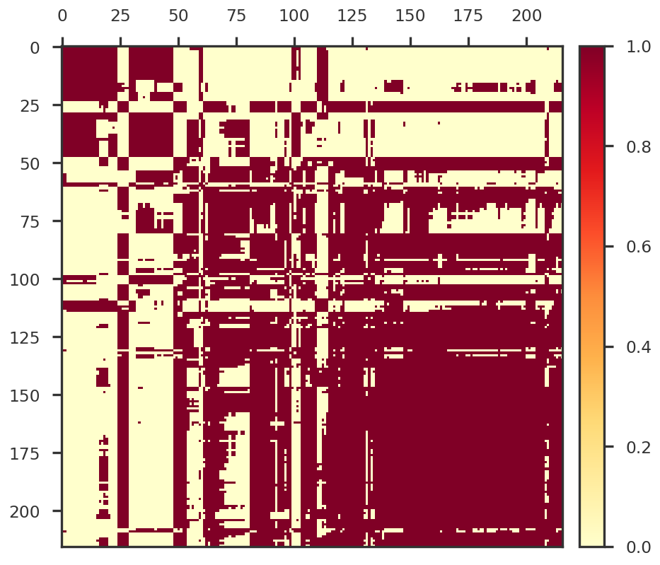
In Figure 1 we plot a heatmap from the covariance matrix of the Z-scores.

Code

o1 = sp_hierarchy.leaves_list(sp_hierarchy.linkage(np.cov(X_cent), method = 'centroid'))

fig = plt.figure(figsize = (8, 8))
ax1 = fig.add_subplot(111)

mpy_plotfn.plot_covariance_heatmap(ax1, X_cent[o1, :])

plt.tight_layout()
plt.show()

Figure 1: Covariance of Z-scores in PanUKB data

Code

method_labels = {
    "rpca" : "RPCA-IALM",
    "nnm" : "NN-FW",
    "nnm_sparse" : "NN-Sparse-FW",
    "truncated_svd": "tSVD",
    "factorgo": "FactorGO",
}

method_colors = {
    "rpca" : '#FF6800', # Vivid Orange
    "nnm" : '#C10020', # Vivid Red
    "nnm_sparse" : '#803E75', # Strong Purple
    "truncated_svd" : '#535154', # gray
    "factorgo" : '#A6BDD7', # Very Light Blue
}

optimum_rmse = dict()

Read RPCA results

Code

rpca_filename = os.path.join(dscout_dir, f"rpca/ukbb_1_rpca_1.pkl")
    
with (open(rpca_filename, "rb")) as fh:
    rpca_res = pickle.load(fh)
    
optimum_rmse['rpca'] = get_masked_rmse(X_cent, rpca_res['X'], mask = Z_mask)

To find the best possible lambda, we apply Robust PCA on the masked data with different values of \lambda. The RMSE of the recovered values is shown in Figure 2. As currently implemented, Robust PCA fails to recover the masked data and the RMSE is comparable to that from zero entries.

Code

fig = plt.figure()
ax1 = fig.add_subplot(111)

_optlmb = rpca_res['cvlmb'][np.argmin(rpca_res['cvrmse'])]

ax1.plot(rpca_res['cvlmb'], rpca_res['cvrmse'], marker = 'o')
ax1.axvline(x = _optlmb, ls = 'dotted', color = 'grey')
ax1.set_xlabel("Lambda")
ax1.set_ylabel("RMSE for masked entries")
plt.show()

Figure 2: RMSE of recovered values of masked entries in the PanUKB data

Read NNM results

Code

nnm_filename = os.path.join(dscout_dir, f"nnm/ukbb_1_nnm_1.pkl")
    
with (open(nnm_filename, "rb")) as fh:
    nnm_res = pickle.load(fh)

For NNM, we consider the input as an incomplete data matrix. We perform a 2-fold cross-validation on the incomplete input data and show the RMSE for the CV and the RMSE for the cross-validation is shown in Figure 3.

Code

fig = plt.figure()
ax1 = fig.add_subplot(111)

nnm_cvres = nnm_res['model']['test_error']

ax1.plot(nnm_cvres.keys(), [np.mean(x) for x in nnm_cvres.values()], marker = 'o')
ax1.set_xlabel("Nuclear Norm Cutoff")
ax1.set_ylabel("Cross validation RMSE")
plt.show()

Figure 3: RMSE for recovery of hold-out test data

Read NNM Sparse results

Code

rank_seq = [128.0, 256.0, 512.0, 1024.0, 2048.0, 4096.0, 8192.0, 16384.0, 32768.0, 65536.0]
nnm_sparse_res = dict()
for r in rank_seq:
    out_filename = os.path.join(dscout_dir, f"nnm_sparse/ukbb_1_nnm_sparse_{r}.pkl")
    if os.path.isfile(out_filename):
        with open(out_filename, 'rb') as fh:
            nnm_sparse_res[r] = pickle.load(fh)

Code

nnm_sparse_cvres = dict()
nnm_sparse_nucnorm = dict()
for rank, model in nnm_sparse_res.items():
    nnm_sparse_cvres[rank] = get_masked_rmse(X_cent, model['X_'], mask = Z_mask)
    nnm_sparse_nucnorm[rank] = np.linalg.norm(model['X_'], 'nuc')

For the NNM Sparse model, we looked at the RMSE of the masked data predicted by NNM in the left panel of Figure 4. In the right panel, we show the nuclear norm of the recovered matrix against the input constraint.

Code

fig = plt.figure(figsize = (14,6))
ax1 = fig.add_subplot(121)
ax2 = fig.add_subplot(122)

ax1.plot(nnm_sparse_cvres.keys(), nnm_sparse_cvres.values(), marker = 'o')
# ax1.plot(nnm_sparse_nucnorm.values(), nnm_sparse_cvres.values(), marker = 'o')
# ax1.plot(nnm_cvres.keys(), [np.mean(x) * 1.11 for x in nnm_cvres.values()], marker = 'o')
ax1.set_xlabel("Nuclear Norm Cutoff")
ax1.set_ylabel("RMSE")

ax2.plot(nnm_sparse_nucnorm.keys(), nnm_sparse_nucnorm.values(), marker = 'o')
ax2.set_xlabel("Nuclear Norm Cutoff")
ax2.set_ylabel("Nuclear Norm Observed")
mpl_utils.plot_diag(ax2)

plt.tight_layout(w_pad = 4.0)
plt.show()

Figure 4: RMSE for masked data in the UK Biobank decreases with increasing rank.

Code

nnm_sparse_filename = os.path.join(dscout_dir, f"nnm_sparse/ukbb_1_nnm_sparse_1.pkl")
    
with (open(nnm_sparse_filename, "rb")) as fh:
    nnm_sparse_res = pickle.load(fh)

Code

optimum_rmse['nnm'] = get_masked_rmse(X_cent, nnm_res['X'], mask = Z_mask)
optimum_rmse['nnm_sparse'] = get_masked_rmse(X_cent, nnm_sparse_res['X'], mask = Z_mask)

Truncated SVD

Code

def truncated_svd(X, k):
    #X_cent = X - np.mean(X, axis = 0, keepdims = True)
    #X_cent /= np.sqrt(np.prod(X_cent.shape))
    #U, S, Vt = np.linalg.svd(X_cent, full_matrices = False)
    U, S, Vt = np.linalg.svd(X, full_matrices = False)
    U = U[:, 0:k]
    S = S[0:k]
    V = Vt.T
    V = V[:, 0:k]
    L = U @ np.diag(S)
    F = V @ np.diag(S)
    S2 = np.square(S)
    #return L, F, S2
    return L @ F.T

tsvd_X = truncated_svd(Z_cent, 100)

# X_cent_pr, tsvd_X_pr, _ = sp_procrustes(X_cent, tsvd_X)

Code

fig = plt.figure(figsize = (8, 8))
ax1 = fig.add_subplot(111)

mpy_plotfn.plot_covariance_heatmap(ax1, tsvd_X[o1, :])

plt.tight_layout()
plt.show()

Figure 5: Covariance of Z-scores recovered using truncated SVD

Visualize the correlation matrix with only the masked entries

Code

fig = plt.figure(figsize = (16, 16))
ax1 = fig.add_subplot(221)
ax2 = fig.add_subplot(222)
ax3 = fig.add_subplot(223)
ax4 = fig.add_subplot(224)

X_cent_masked = X_cent.copy()
X_cent_masked[~Z_mask] = 0.0

rpca_X_masked = np.zeros_like(X_cent)
rpca_X_masked[Z_mask] = rpca_res['X'][Z_mask]

nnm_X_masked = np.zeros_like(X_cent)
nnm_X_masked[Z_mask] = nnm_res['X'][Z_mask]

nnm_sparse_X_masked = np.zeros_like(X_cent)
nnm_sparse_X_masked[Z_mask] = nnm_sparse_res['X'][Z_mask]


vmax = 0.4
mpy_plotfn.plot_covariance_heatmap(ax1, X_cent_masked[o1, :], vmax = vmax)
mpy_plotfn.plot_covariance_heatmap(ax2, rpca_X_masked[o1, :], vmax = vmax)
mpy_plotfn.plot_covariance_heatmap(ax3, nnm_X_masked[o1, :], vmax = vmax)
mpy_plotfn.plot_covariance_heatmap(ax4, nnm_sparse_X_masked[o1, :], vmax = vmax)

ax1.set_title("Masked entries", pad = 20)
ax2.set_title("RPCA", pad = 20)
ax3.set_title("NN-FW", pad = 20)
ax4.set_title("NN-Sparse-FW", pad = 20)

for ax in [ax1, ax2, ax3, ax4]:
    ax.tick_params(left = False, top = False, labelleft=False, labeltop=False)

plt.tight_layout()
plt.show()

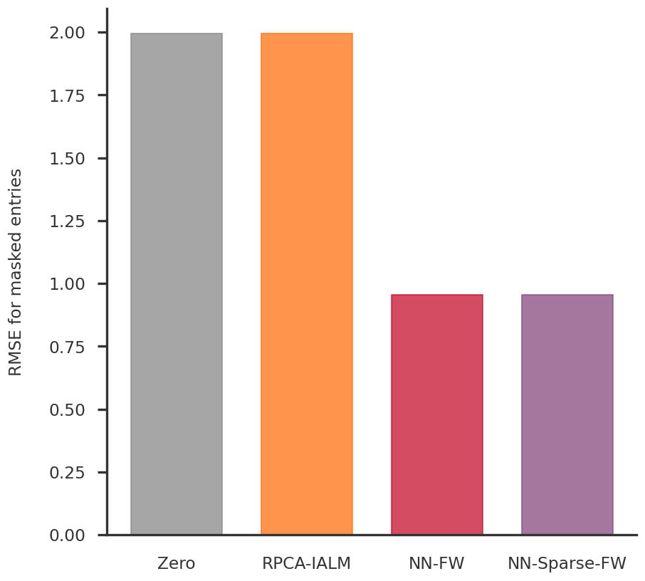
Figure 6: Correlation of Z-scores for the masked entries recovered by the different methods.

Code

fig = plt.figure(figsize = (8, 8))
ax1 = fig.add_subplot(111)

yvals = [get_masked_rmse(X_cent, Z_cent, mask=Z_mask)] + list(optimum_rmse.values())
xvals = np.arange(len(yvals))
bcolors = ["grey"] + [method_colors[x] for x in optimum_rmse.keys()]

ax1.bar(xvals, yvals, align = 'center', width = 0.7, color = bcolors, edgecolor = bcolors, alpha = 0.7)
ax1.set_xticks(xvals)
ax1.set_xticklabels(["Zero"] + [method_labels[x] for x in optimum_rmse.keys()])

for side in ['top', 'right']:
    ax1.spines[side].set_visible(False)
    
ax1.tick_params(bottom=False)
ax1.set_ylabel("RMSE for masked entries")

plt.show()

Figure 7: RMSE for recovery of masked entries