Pan-UKB Principal Components v01

Author

Saikat Banerjee

Published

December 8, 2023

Abstract

We look at the first few principal components of the low rank matrix obtained by applying our method on the z-scores of Pan-UKB summary statistics.

Code

import numpy as np
import pandas as pd
import pickle

import matplotlib.pyplot as plt
from pymir import mpl_stylesheet
from pymir import mpl_utils
mpl_stylesheet.banskt_presentation(splinecolor = 'black', dpi = 120, colors = 'kelly')
from matplotlib.gridspec import GridSpec

from nnwmf.optimize import IALM
from nnwmf.optimize import FrankWolfe, FrankWolfe_CV
from nnwmf.utils import model_errors as merr

import sys
sys.path.append("../utils/")
import simulate as mpy_simulate

Read Data and Results

Code

data_dir = "/gpfs/commons/home/sbanerjee/work/npd/PanUKB/data"
result_dir = "/gpfs/commons/home/sbanerjee/work/npd/PanUKB/nnwmf"
zscore_filename = f"{data_dir}/GWAS_Zscore.tsv"
trait_filename = f"{data_dir}/trait_manifest_TableS6_no_readme.tsv"
zscore_df = pd.read_csv(zscore_filename, sep = '\t')
trait_df = pd.read_csv(trait_filename, sep = '\t')

# remove extra columns from trait_df

colnames = trait_df.columns.tolist()
colnames[0] = "zindex"
trait_df.columns = colnames
trait_df_mod = trait_df.drop(labels = ['coding', 'modifier', 'coding_description', 'filename', 'aws_link'], axis=1)
trait_df_mod

zscore_df

	rsid	z1	z2	z3	z4	z5	z6	z7	z8	z9	...	z2474	z2475	z2476	z2477	z2478	z2479	z2480	z2481	z2482	z2483
0	rs6657440	-0.903532	0.561842	0.711068	-0.109174	0.223668	-1.728199	0.374988	-0.265971	-2.823282	...	1.521092	0.612532	1.405428	0.018029	0.895337	-0.008761	-2.069432	-4.292948	-4.701711	2.952899
1	rs7418179	0.398166	1.163539	0.512118	0.144794	-1.313903	-1.547410	0.450270	0.560324	-1.502268	...	-0.296537	-0.734266	-0.093081	0.412077	1.961159	0.716049	-2.171984	-5.314085	-6.612137	3.817518
2	rs80125161	-1.739115	-0.172328	0.349145	-0.329335	-0.870640	-1.004155	1.128148	0.151244	-1.816075	...	2.222433	1.092969	2.328233	1.160767	0.909524	-1.467249	-0.135785	-2.187241	-3.223529	4.508578
3	rs7524174	-0.884478	-1.762000	1.312823	-0.550764	2.132540	0.519828	0.834194	0.699441	-0.885281	...	3.356354	1.990588	3.092179	-0.133810	-0.072845	-1.376310	1.317044	0.913491	0.535188	2.245657
4	rs3829740	-1.469931	-0.519628	-0.281605	-0.267729	-1.060167	0.058116	-0.638319	-0.589767	0.228514	...	-0.320075	-0.128047	-0.524757	-0.232900	-1.051020	-0.483644	2.026508	4.400092	5.407316	1.125536
...	...	...	...	...	...	...	...	...	...	...	...	...	...	...	...	...	...	...	...	...	...
51394	rs9616937	-0.211947	1.371231	-1.800776	0.609980	-0.619822	0.947269	-1.166021	0.478601	-0.359714	...	0.714167	0.354347	0.611158	-0.354725	1.073043	-0.831737	0.870924	1.432076	2.228501	0.536104
51395	rs1024374	0.027097	-1.817082	0.530216	0.813498	-0.076514	0.784427	1.411160	-1.111740	-0.224438	...	1.107098	1.482684	1.512723	0.322355	-0.374603	1.320194	-0.700092	-1.395039	-2.270186	0.360025
51396	rs144480800	0.545682	0.391830	0.520505	-1.280976	0.453876	-1.388940	0.025094	0.737788	1.178641	...	-0.562063	-1.148515	-0.994185	-0.268232	-0.069619	0.013256	-0.777667	-1.544760	-1.406344	2.205817
51397	rs5770994	1.441851	1.152368	-1.500000	-0.468137	-0.444156	-0.780139	-0.853550	-0.316097	0.311219	...	-1.185702	-0.624073	-0.859522	0.549669	1.809912	0.268733	0.947441	1.533302	1.658537	2.218653
51398	rs9616824	0.669372	-0.308184	-0.811311	-0.154224	1.476823	0.065167	-1.030063	-0.215723	-0.631385	...	0.308486	0.612102	0.492977	-0.621278	-2.657386	-0.732402	-0.106474	-0.029006	0.070647	-0.805253

51399 rows × 2484 columns

Code

X_nan = np.array(zscore_df.loc[:, zscore_df.columns!='rsid']).T
X_nan_cent = X_nan - np.nanmean(X_nan, axis = 0, keepdims = True)
X_nan_mask = np.isnan(X_nan)
X_cent = np.nan_to_num(X_nan_cent, copy = True, nan = 0.0)

print (f"We have {X_cent.shape[0]} samples (phenotypes) and {X_cent.shape[1]} features (variants)")
print (f"Fraction of Nan entries: {np.sum(X_nan_mask) / np.prod(X_cent.shape):.3f}")

We have 2483 samples (phenotypes) and 51399 features (variants)
Fraction of Nan entries: 0.000

Code

mf_methods = ['ialm', 'nnm_sparse', 'tsvd']

method_prefix = {
    'ialm' : 'ialm_maxiter10000_admm',
    'nnm_sparse' : 'nnm_sparse_maxiter1000'
}

method_names = {
    'tsvd' : 'Raw Data',
    'ialm' : 'RPCA-IALM',
    'nnm'  : 'NNM-FW',
    'nnm_weighted' : 'NNM-Weighted',
    'nnm_sparse' : 'NNM-Sparse-FW',
}

with open (f"{result_dir}/{method_prefix['ialm']}_progress.pkl", 'rb') as handle:
    ialm = pickle.load(handle)
    
with open (f"{result_dir}/{method_prefix['nnm_sparse']}_progress.pkl", 'rb') as handle:
    nnm_sparse = pickle.load(handle)

Convergence of low rank approximations

In the following two figures, Figure 1 and Figure 2, we look at the convergence properties of the different methods on the Pan-UKB dataset.

Code

fig = plt.figure(figsize = (20, 6))
ax1 = fig.add_subplot(121)
ax2 = fig.add_subplot(122)

ax1.plot(range(len(ialm['mu_list'])), ialm['mu_list'], 'o-', label = 'ADMM')
ax1.legend()
ax1.set_xlabel("Iteration")
ax1.set_ylabel("Step size")

ax2.plot(range(len(ialm['primal_residual'])),   np.log10(ialm['primal_residual']),   label = 'Primal Residual')
ax2.plot(range(len(ialm['dual_residual']) - 1), np.log10(ialm['dual_residual'][1:]), label = 'Dual Residual')
ax2.legend()
ax2.set_xlabel("Iteration")
ax2.set_ylabel("Primal and Dual Residuals (log10 scale)")

plt.tight_layout(w_pad = 2.0)
plt.show()

Figure 1: Convergence properties of Robust PCA using IALM.

Code

fig = plt.figure(figsize = (20, 6))
ax1 = fig.add_subplot(121)
ax2 = fig.add_subplot(122)

ax1.plot(range(len(nnm_sparse['steps'])), nnm_sparse['steps'])
# ax1.legend()
ax1.set_xlabel("Iteration")
ax1.set_ylabel("Step size")

ax2b = ax2.twinx()
colors = mpl_stylesheet.kelly_colors()
#p1 = ax2.plot(range(len(nnm_sparse['objective']) - 2), - np.diff(nnm_sparse['objective'])[1:], 'o-', label = 'Objective', color = colors[0])
p1 = ax2.plot(range(len(nnm_sparse['objective']) - 1), nnm_sparse['objective'][1:], label = 'Objective', color = colors[0])
p2 = ax2b.plot(range(len(nnm_sparse['duality_gap']) - 2), nnm_sparse['duality_gap'][2:], label = 'Duality Gap', color = colors[1])

ax2.set_xlabel("Iteration")
ax2.set_ylabel("Objective Function")
ax2.yaxis.label.set_color(p1[0].get_color())
ax2b.set_ylabel("Duality Gap")
ax2b.yaxis.label.set_color(p2[0].get_color())

plt.tight_layout(w_pad = 2.0)
plt.show()

Figure 2: Convergence properties of sparse Nuclear Norm matrix factorization using Frank-Wolfe algorithm

PCA of Low Rank Matrix

Code

def get_principal_components(X):
    X_cent = mpy_simulate.do_standardize(X, scale = False)
    X_cent /= np.sqrt(np.prod(X_cent.shape))
    U, S, Vt = np.linalg.svd(X_cent, full_matrices = False)
    pcomps = U @ np.diag(S)
    loadings = Vt.T @ np.diag(S)
    return loadings, pcomps, S

lowrank_X = dict()
loadings  = dict()
pcomps    = dict()
eigenvals = dict()

for m in mf_methods:
    if m != 'tsvd':
        with open (f"{result_dir}/{method_prefix[m]}_lowrank_X.pkl", 'rb') as handle:
            lowrank_X[m] = pickle.load(handle)
lowrank_X['tsvd'] = X_cent.copy()
for m in mf_methods:
    loadings[m], pcomps[m], eigenvals[m] = get_principal_components(lowrank_X[m])

Nuclear Norm of Low Rank Matrix

Code

for m in mf_methods:
    print (f"{method_names[m]}: {np.linalg.norm(lowrank_X[m], 'nuc'):g}")

RPCA-IALM: 180216
NNM-Sparse-FW: 1023.04
Raw Data: 495872

L0 norm of error matrix

Code

lowrank_E = dict()
for m in mf_methods:
    if m != 'tsvd':
        with open (f"{result_dir}/{method_prefix[m]}_lowrank_E.pkl", 'rb') as handle:
            lowrank_E[m] = pickle.load(handle)

Code

for m in mf_methods:
    if m != 'tsvd':
        print (f"{method_names[m]}: {np.linalg.norm(lowrank_E[m], ord = 1):g}")
    else:
        print (f"{method_names[m]}: {np.linalg.norm(lowrank_X[m], ord = 1):g}")

RPCA-IALM: 2003.58
NNM-Sparse-FW: 3491.56
Raw Data: 4527.88

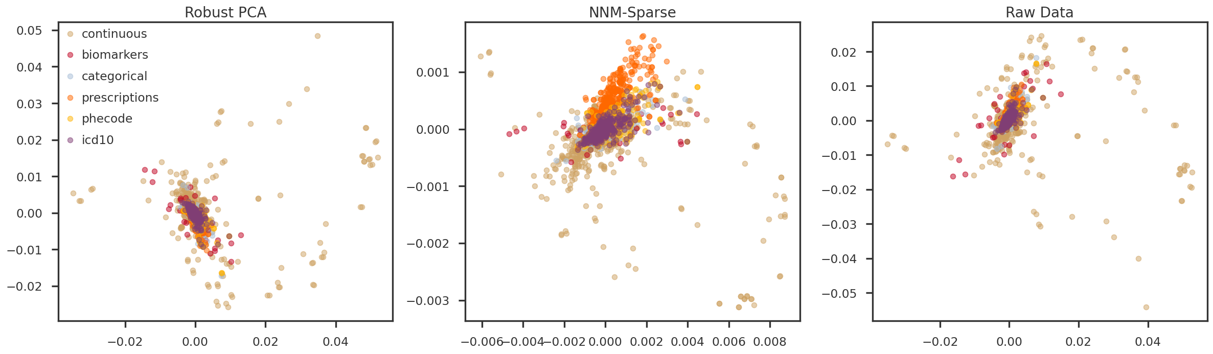
Plots for Principal Components (Hidden Factors)

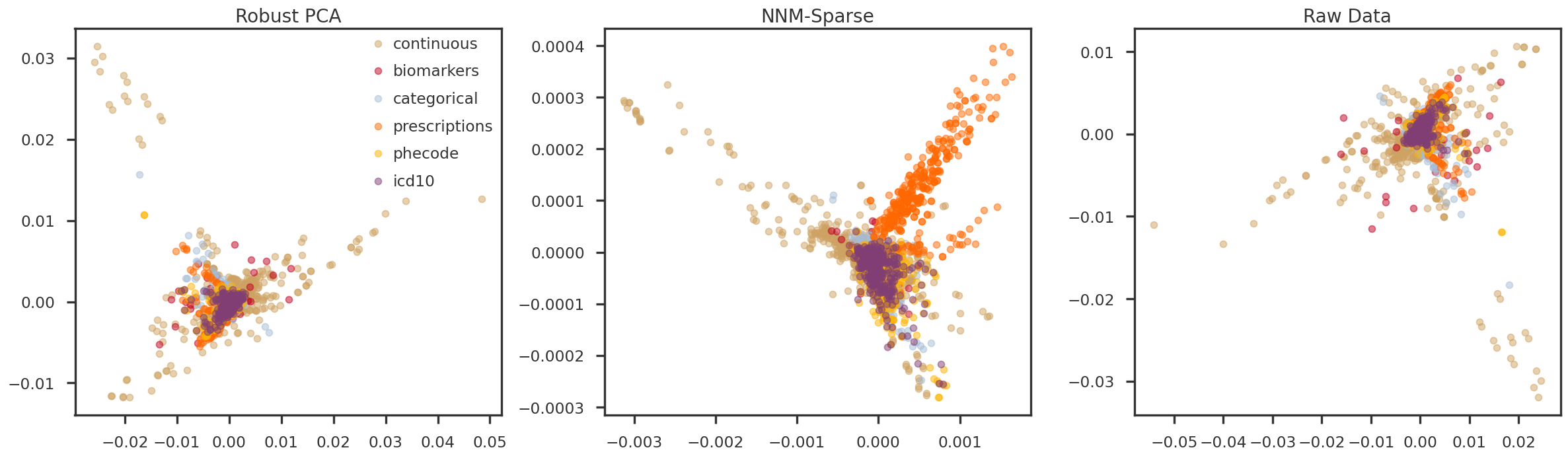
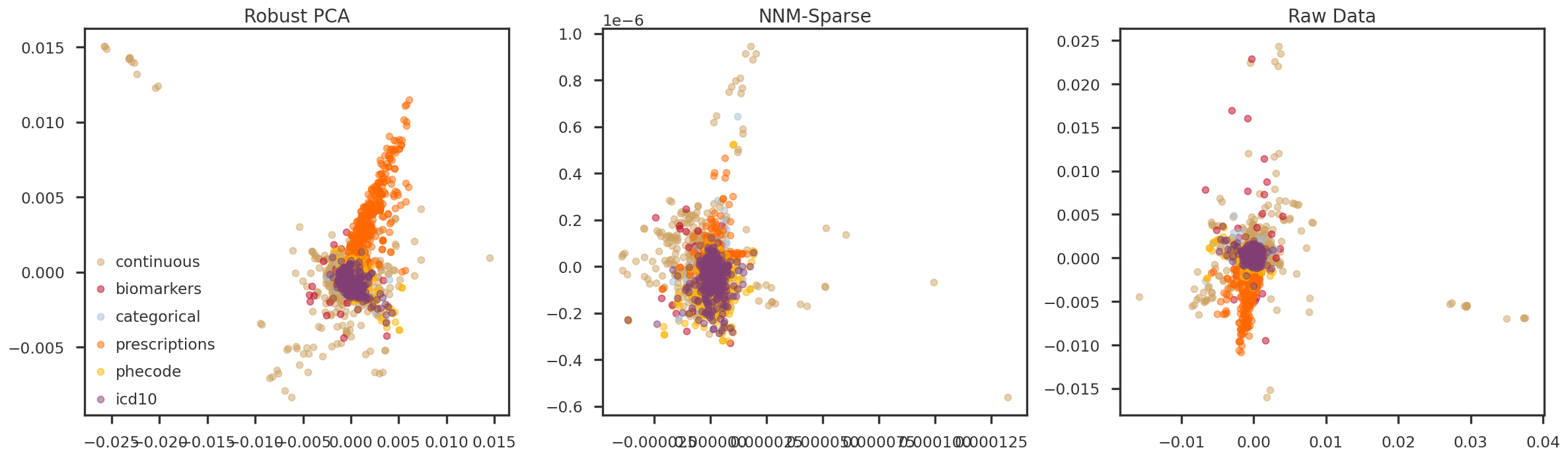
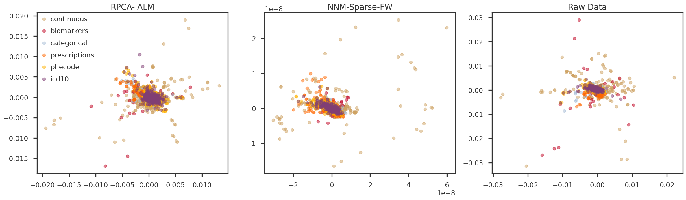
In the following figures, we look at the first few principal components (hidden factors) obtained by applying PCA on the predicted low-rank matrices. The samples are colored using the six trait types for the Pan-UKB project. They are: - continuous: Quantitative traits obtained from questionnaires and assessment centers, e.g. standing height, distance between home and job workplace, etc. - biomarkers: Obtained from biological samples, e.g. cholesterol, triglycerides. - prescriptions: Varied treatment/medication/prescriptions, e.g. amoxicillin, corticosteroids, etc. - icd10: Set of ICD10 codes - phecode: PHESANT software? Manually curated by FinnGen? - categorical: Categorical traits obtained from questionnaires and assessment centers, e.g. different self-reported illness, COVID-19, self-reported treatment/medication, etc.

Code

trait_types  = trait_df_mod['trait_type'].unique().tolist()
trait_colors = {trait: color for trait, color in zip(trait_types, mpl_stylesheet.kelly_colors()[:len(trait_types)])}
trait_types.reverse()

Code

fig = plt.figure(figsize = (20, 6))
ax = [None for m in mf_methods]

ipc1 = 0
ipc2 = 1

for i, m in enumerate(mf_methods):
    ax[i] = fig.add_subplot(1, 3, i+1)
    for t in trait_types:
        tidx = np.array(trait_df_mod[trait_df_mod['trait_type'] == t].index)
        ax[i].scatter(pcomps[m][tidx, ipc1], pcomps[m][tidx, ipc2], alpha = 0.5, color = trait_colors[t], label = t)
    ax[i].set_title(method_names[m])
    if i == 0:
        ax[i].legend()
    
plt.tight_layout(h_pad = 2.0)
plt.show()

Code

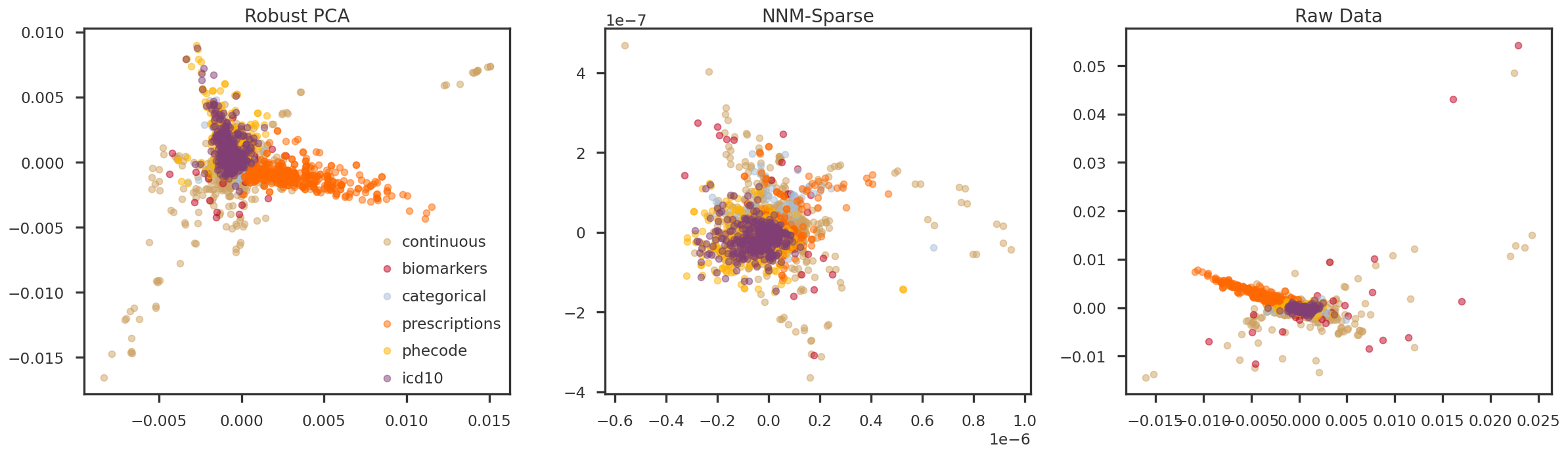
fig = plt.figure(figsize = (20, 6))
ax = [None for m in mf_methods]

ipc1 = 1
ipc2 = 2

for i, m in enumerate(mf_methods):
    ax[i] = fig.add_subplot(1, 3, i+1)
    for t in trait_types:
        tidx = np.array(trait_df_mod[trait_df_mod['trait_type'] == t].index)
        ax[i].scatter(pcomps[m][tidx, ipc1], pcomps[m][tidx, ipc2], alpha = 0.5, color = trait_colors[t], label = t)
    ax[i].set_title(method_names[m])
    if i == 0:
        ax[i].legend()
    
plt.tight_layout(h_pad = 2.0)
plt.show()

Code

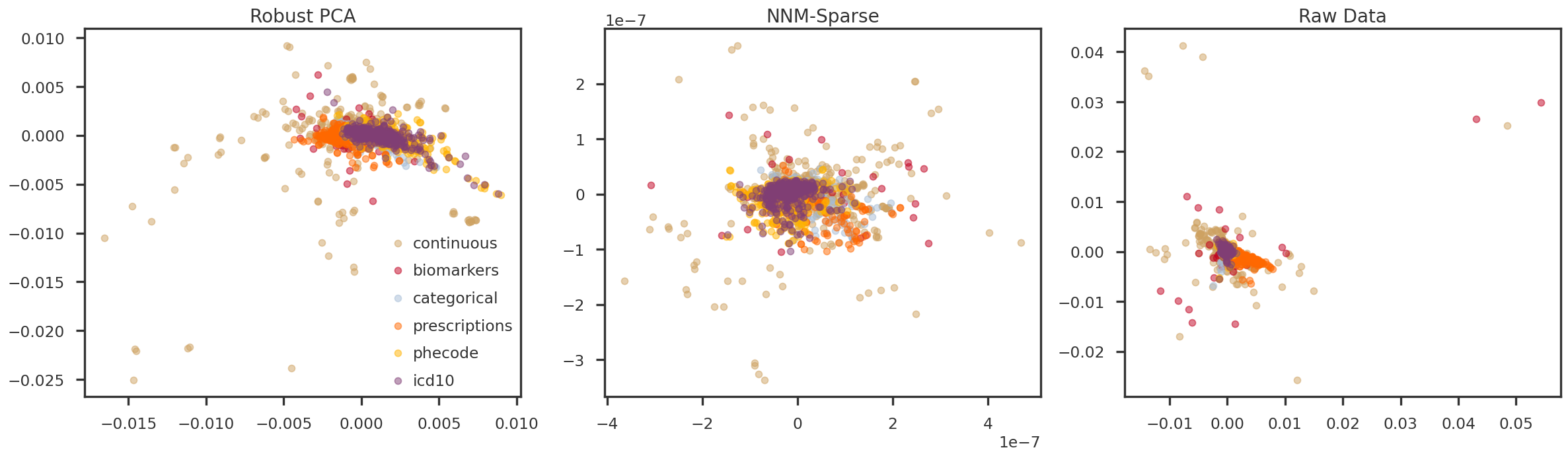
fig = plt.figure(figsize = (20, 6))
ax = [None for m in mf_methods]

ipc1 = 2
ipc2 = 3

for i, m in enumerate(mf_methods):
    ax[i] = fig.add_subplot(1, 3, i+1)
    for t in trait_types:
        tidx = np.array(trait_df_mod[trait_df_mod['trait_type'] == t].index)
        ax[i].scatter(pcomps[m][tidx, ipc1], pcomps[m][tidx, ipc2], alpha = 0.5, color = trait_colors[t], label = t)
    ax[i].set_title(method_names[m])
    if i == 0:
        ax[i].legend()
    
plt.tight_layout(h_pad = 2.0)
plt.show()

Code

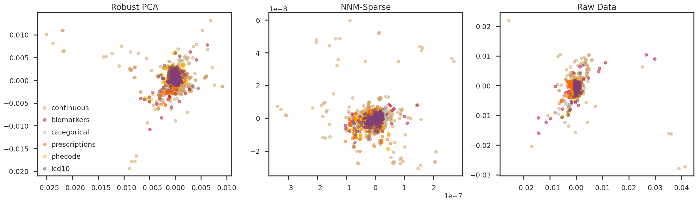
fig = plt.figure(figsize = (20, 6))
ax = [None for m in mf_methods]

ipc1 = 3
ipc2 = 4

for i, m in enumerate(mf_methods):
    ax[i] = fig.add_subplot(1, 3, i+1)
    for t in trait_types:
        tidx = np.array(trait_df_mod[trait_df_mod['trait_type'] == t].index)
        ax[i].scatter(pcomps[m][tidx, ipc1], pcomps[m][tidx, ipc2], alpha = 0.5, color = trait_colors[t], label = t)
    ax[i].set_title(method_names[m])
    if i == 0:
        ax[i].legend()
    
plt.tight_layout(h_pad = 2.0)
plt.show()

Code

fig = plt.figure(figsize = (20, 6))
ax = [None for m in mf_methods]

ipc1 = 4
ipc2 = 5

for i, m in enumerate(mf_methods):
    ax[i] = fig.add_subplot(1, 3, i+1)
    for t in trait_types:
        tidx = np.array(trait_df_mod[trait_df_mod['trait_type'] == t].index)
        ax[i].scatter(pcomps[m][tidx, ipc1], pcomps[m][tidx, ipc2], alpha = 0.5, color = trait_colors[t], label = t)
    ax[i].set_title(method_names[m])
    if i == 0:
        ax[i].legend()
    
plt.tight_layout(h_pad = 2.0)
plt.show()

Code

fig = plt.figure(figsize = (20, 6))
ax = [None for m in mf_methods]

ipc1 = 5
ipc2 = 6

for i, m in enumerate(mf_methods):
    ax[i] = fig.add_subplot(1, 3, i+1)
    for t in trait_types:
        tidx = np.array(trait_df_mod[trait_df_mod['trait_type'] == t].index)
        ax[i].scatter(pcomps[m][tidx, ipc1], pcomps[m][tidx, ipc2], alpha = 0.5, color = trait_colors[t], label = t)
    ax[i].set_title(method_names[m])
    if i == 0:
        ax[i].legend()
    
plt.tight_layout(h_pad = 2.0)
plt.show()

Code

fig = plt.figure(figsize = (20, 6))
ax = [None for m in mf_methods]

ipc1 = 6
ipc2 = 7

for i, m in enumerate(mf_methods):
    ax[i] = fig.add_subplot(1, 3, i+1)
    for t in trait_types:
        tidx = np.array(trait_df_mod[trait_df_mod['trait_type'] == t].index)
        ax[i].scatter(pcomps[m][tidx, ipc1], pcomps[m][tidx, ipc2], alpha = 0.5, color = trait_colors[t], label = t)
    ax[i].set_title(method_names[m])
    if i == 0:
        ax[i].legend()
    
plt.tight_layout(h_pad = 2.0)
plt.show()

Code

fig = plt.figure(figsize = (20, 6))
ax = [None for m in mf_methods]

ipc1 = 7
ipc2 = 8

for i, m in enumerate(mf_methods):
    ax[i] = fig.add_subplot(1, 3, i+1)
    for t in trait_types:
        tidx = np.array(trait_df_mod[trait_df_mod['trait_type'] == t].index)
        ax[i].scatter(pcomps[m][tidx, ipc1], pcomps[m][tidx, ipc2], alpha = 0.5, color = trait_colors[t], label = t)
    ax[i].set_title(method_names[m])
    if i == 0:
        ax[i].legend()
    
plt.tight_layout(h_pad = 2.0)
plt.show()

Code

fig = plt.figure(figsize = (20, 6))
ax = [None for m in mf_methods]

ipc1 = 8
ipc2 = 9

for i, m in enumerate(mf_methods):
    ax[i] = fig.add_subplot(1, 3, i+1)
    for t in trait_types:
        tidx = np.array(trait_df_mod[trait_df_mod['trait_type'] == t].index)
        ax[i].scatter(pcomps[m][tidx, ipc1], pcomps[m][tidx, ipc2], alpha = 0.5, color = trait_colors[t], label = t)
    ax[i].set_title(method_names[m])
    if i == 0:
        ax[i].legend()
    
plt.tight_layout(h_pad = 2.0)
plt.show()