Stability heatmaps for PGC split-replication CV

Author

Saikat Banerjee

Published

April 30, 2026

Abstract
Visualize split-replication stability metrics from the Clorinn cross-validation pipeline. The notebook reads per-radius JSON summaries, converts by-k metrics into k-by-nuclear-norm grids, and plots heatmaps for projection distance, cumulative singular-value energy, and largest principal angle.
Code
import json
import pickle
from pathlib import Path
import numpy as np
import pandas as pd

import matplotlib.pyplot as plt
from pymir import mpl_stylesheet
from pymir import mpl_utils
mpl_stylesheet.banskt_presentation(splinecolor = 'black', dpi = 300, fontsize=14)

from matplotlib import colormaps as mpl_cmaps
import matplotlib.colors as mpl_colors
from mpl_toolkits.axes_grid1 import make_axes_locatable

Paths and analysis settings

data_root should point to the Snakemake output directory for the split-replication CV run. The notebook expects:

  • per-radius stability JSON files under stability/
  • the aggregate stability metric CSV under summary/

prefix identifies the model/solver combination. For example, pgd_fw_nnm matches files such as pgd_fw_nnm_r8192.json.

Code
data_root = "/gpfs/commons/groups/knowles_lab/data/PsychGen/analysis/clorinn/cv_split_replication"
# Model/solver prefix used by the Snakemake output filenames.
PREFIXES = ["pgd_afw_nnm_corr", "pgd_fw_nnm"]

stability_out_dir = f"{data_root}/stability"
summary_out = f"{data_root}/summary/{PREFIXES[0]}_stability_metrics.csv"

fig_dir = Path("figures/split_replication_cv")
fig_dir.mkdir(parents=True, exist_ok=True)

Read aggregate summary table

This CSV is not required for the heatmaps below, but displaying it is a useful sanity check that the expected pipeline outputs were generated.

Code
summary_df = pd.read_csv(summary_out)
summary_df.head()
nucnorm mean_dist_k1 mean_dist_k2 mean_dist_k3 mean_dist_k4 mean_dist_k5 mean_dist_k6 mean_dist_k7 mean_dist_k8 mean_dist_k9 ... se_energy_k22 se_energy_k23 se_energy_k24 se_energy_k25 se_energy_k26 se_energy_k27 se_energy_k28 se_energy_k29 se_energy_k30 grid
0 1.0 0.021770 0.203261 0.529161 0.600799 0.648400 0.660207 0.659052 0.660754 0.667229 ... 0.0 0.0 0.0 0.0 0.0 0.0 0.0 0.0 0.0 coarse
1 2.0 0.022354 0.274409 0.577392 0.564718 0.588592 0.624654 0.654132 0.668207 0.659147 ... 0.0 0.0 0.0 0.0 0.0 0.0 0.0 0.0 0.0 coarse
2 4.0 0.023633 0.266199 0.536371 0.635676 0.662308 0.665486 0.668800 0.676398 0.675788 ... 0.0 0.0 0.0 0.0 0.0 0.0 0.0 0.0 0.0 coarse
3 8.0 0.026768 0.326992 0.566602 0.625170 0.634612 0.643133 0.661838 0.670966 0.670403 ... 0.0 0.0 0.0 0.0 0.0 0.0 0.0 0.0 0.0 coarse
4 16.0 0.034373 0.054074 0.169477 0.484521 0.601823 0.635789 0.658699 0.674419 0.663070 ... 0.0 0.0 0.0 0.0 0.0 0.0 0.0 0.0 0.0 coarse

5 rows × 152 columns

Helper functions

The stability JSON files are stored one file per radius. Each file contains a by_k list with metrics evaluated at several ranks. The helper functions below convert this nested JSON structure into rectangular matrices suitable for heatmaps.

Code
def load_stability_jsons(stability_dir, prefix):
    stability_dir = Path(stability_dir)
    paths = sorted(stability_dir.glob(f"{prefix}_r*.json"))

    records = []
    for path in paths:
        with open(path) as fh:
            rec = json.load(fh)
        rec["_path"] = str(path)
        records.append(rec)

    return records


def build_by_k_metrics_grid(records, metric, *, duplicate="error"):
    rows = []

    for rec in records:
        nucnorm = int(round(float(rec["nucnorm_full"])))

        for entry in rec["by_k"]:
            value = entry[metric]
            rows.append({
                "nucnorm": nucnorm, 
                "k": int(entry["k"]), 
                metric: float(value),
            })

    long_df = pd.DataFrame(rows)

    dup_mask = long_df.duplicated(subset=["nucnorm", "k"], keep=False)
    # Look for duplicates. This can happen if coarse and fine grids
    # contain the same nucnorm.
    if dup_mask.any():
        keep = "first" if duplicate == "first" else "last"
        long_df = (
            long_df
            .sort_values(["nucnorm", "k"])
            .drop_duplicates(subset=["nucnorm", "k"], keep=keep)
        )
    grid_df = (
        long_df
        .pivot(index="k", columns="nucnorm", values=metric)
        .sort_index(axis=0)
        .sort_index(axis=1)
    )

    grid_df.index.name = "k"
    grid_df.columns.name = "nucnorm"

    return grid_df

Load stability metrics as heatmap grids

The three metrics below summarize complementary aspects of split-replication stability:

  • mean_dist: mean projection distance between the top-k trait subspaces from two SNP splits. Lower is more stable.
  • mean_energy: mean cumulative singular-value energy captured by the top-k directions. Higher means the selected k captures more fitted signal.
  • mean_gap_angle: mean largest principal angle between split-specific top-k subspaces. Lower angles indicate more similar subspaces.

For plotting, duplicate radii are resolved with duplicate="first" because the coarse and fine radius grids can overlap.

Code
records      = load_stability_jsons(stability_out_dir, PREFIXES[0])
dist_df      = build_by_k_metrics_grid(records, "mean_dist", duplicate="first")
energy_df    = build_by_k_metrics_grid(records, "mean_energy", duplicate="first")
gap_angle_df = build_by_k_metrics_grid(records, "mean_gap_angle", duplicate="first")

Sanity check: projection-distance grid

Inspect the main metric before plotting. Rows are ranks k; columns are nuclear-norm radii r.

Code
dist_df
nucnorm 1 2 4 8 16 32 64 128 256 512 ... 4096 8192 9742 11585 13777 16384 19484 23170 27554 32768
k
1 0.021770 0.022354 0.023633 0.026768 0.034373 0.060326 0.279794 0.104825 0.152003 0.316756 ... 0.320522 0.506330 0.501743 0.396054 0.301842 0.215812 0.144993 0.116290 0.095999 0.079928
2 0.203261 0.274409 0.266199 0.326992 0.054074 0.295683 0.086641 0.081347 0.200903 0.353936 ... 0.275586 0.227962 0.246326 0.252714 0.184844 0.165869 0.145464 0.125931 0.106317 0.102684
3 0.529161 0.577392 0.536371 0.566602 0.169477 0.096735 0.076713 0.111989 0.217589 0.190335 ... 0.244471 0.343232 0.201930 0.178022 0.227835 0.247659 0.207810 0.179524 0.164217 0.137322
4 0.600799 0.564718 0.635676 0.625170 0.484521 0.072289 0.145789 0.088911 0.147440 0.208327 ... 0.198169 0.247239 0.255817 0.262621 0.186821 0.171281 0.175579 0.275854 0.315842 0.177260
5 0.648400 0.588592 0.662308 0.634612 0.601823 0.248111 0.067116 0.083585 0.279528 0.250431 ... 0.291562 0.211142 0.248516 0.253508 0.181319 0.158097 0.142910 0.145071 0.145925 0.149781
6 0.660207 0.624654 0.665486 0.643133 0.635789 0.352287 0.171369 0.086962 0.181595 0.190666 ... 0.165505 0.209361 0.387707 0.216801 0.186497 0.184637 0.408319 0.194301 0.135193 0.120031
7 0.659052 0.654132 0.668800 0.661838 0.658699 0.410838 0.248090 0.079737 0.174569 0.226141 ... 0.258335 0.298405 0.213943 0.196292 0.276207 0.281091 0.200430 0.224400 0.216707 0.178804
8 0.660754 0.668207 0.676398 0.670966 0.674419 0.477241 0.395293 0.127913 0.226393 0.209724 ... 0.155959 0.226286 0.180093 0.173730 0.154254 0.290103 0.165114 0.123460 0.110062 0.102487
9 0.667229 0.659147 0.675788 0.670403 0.663070 0.492301 0.325064 0.236133 0.119586 0.216279 ... 0.167974 0.140022 0.133098 0.141958 0.232874 0.125818 0.124066 0.126144 0.130920 0.128427
10 0.663729 0.645370 0.666638 0.665415 0.642089 0.526992 0.286492 0.227014 0.125000 0.203073 ... 0.170039 0.158907 0.159270 0.141397 0.132470 0.149546 0.191185 0.170913 0.137571 0.118974
11 0.653227 0.648982 0.655942 0.663579 0.636723 0.542060 0.315229 0.226680 0.205973 0.229727 ... 0.148883 0.177333 0.296877 0.231520 0.183564 0.144202 0.128840 0.123530 0.126755 0.124764
12 0.647815 0.644796 0.647189 0.657039 0.634875 0.542376 0.401987 0.297775 0.091210 0.172295 ... 0.225370 0.134914 0.133053 0.173915 0.203066 0.138884 0.125501 0.125405 0.138663 0.127219
13 0.645068 0.634569 0.640201 0.655377 0.637249 0.552736 0.414100 0.270003 0.219551 0.185230 ... 0.201447 0.276826 0.130945 0.209423 0.151690 0.146454 0.144382 0.134493 0.109652 0.099926
14 0.639642 0.630299 0.635480 0.646388 0.634297 0.551926 0.417402 0.273897 0.208688 0.178881 ... 0.121710 0.113704 0.154568 0.129166 0.184424 0.250567 0.178167 0.127090 0.111694 0.106479
15 0.637661 0.626039 0.624528 0.632767 0.625635 0.555211 0.424546 0.269076 0.142236 0.123683 ... 0.159821 0.134709 0.138176 0.152514 0.140381 0.170584 0.132584 0.122780 0.110983 0.109904
16 0.633798 0.619918 0.618673 0.623019 0.618064 0.560887 0.457233 0.320675 0.199447 0.134429 ... 0.154963 0.151707 0.123215 0.126346 0.111391 0.093523 0.088187 0.086144 0.087315 0.084148
17 0.633179 0.619101 0.615998 0.619426 0.614817 0.553194 0.473218 0.366062 0.173846 0.150205 ... 0.102382 0.122330 0.139635 0.163327 0.117141 0.120783 0.125901 0.208189 0.114036 0.093891
18 0.626797 0.616877 0.616661 0.618028 0.611843 0.548432 0.474486 0.374961 0.198811 0.154444 ... 0.105974 0.107963 0.154328 0.135993 0.103536 0.121129 0.137080 0.106028 0.107577 0.106659
19 0.622102 0.615457 0.609793 0.616998 0.610163 0.547620 0.483343 0.386162 0.235022 0.167785 ... 0.127883 0.132950 0.119774 0.153111 0.238867 0.120212 0.131742 0.231032 0.136658 0.162114
20 0.619828 0.613809 0.605362 0.613492 0.604743 0.547950 0.490879 0.400664 0.240726 0.231434 ... 0.170172 0.203510 0.129631 0.106692 0.085386 0.078175 0.076375 0.080929 0.108289 0.120661
21 0.614594 0.613430 0.603499 0.611493 0.600098 0.543960 0.497656 0.414459 0.245262 0.206913 ... 0.187105 0.209084 0.157256 0.092092 0.078625 0.078079 0.084960 0.083060 0.080142 0.081833
22 0.610790 0.612906 0.597798 0.608064 0.597299 0.541162 0.500719 0.427059 0.232650 0.192035 ... 0.217630 0.146230 0.125634 0.093102 0.119670 0.120781 0.093612 0.090799 0.111113 0.109520
23 0.607174 0.612037 0.599578 0.603753 0.594936 0.542660 0.503804 0.430821 0.259136 0.192955 ... 0.229208 0.142508 0.192696 0.129440 0.210843 0.175275 0.124295 0.125307 0.107406 0.091736
24 0.602842 0.608530 0.596357 0.599284 0.587992 0.542520 0.511932 0.441961 0.273805 0.198132 ... 0.214826 0.170142 0.173236 0.156336 0.106760 0.106633 0.128976 0.169334 0.125297 0.099436
25 0.602202 0.609923 0.592516 0.592501 0.580094 0.543117 0.508039 0.453017 0.279889 0.129747 ... 0.262111 0.109381 0.120330 0.099806 0.113050 0.127559 0.123499 0.140465 0.158791 0.159888
26 0.598796 0.609891 0.590709 0.591005 0.575211 0.540133 0.510660 0.461997 0.321974 0.203850 ... 0.278312 0.136202 0.120601 0.118398 0.112459 0.121558 0.131622 0.130897 0.125373 0.131924
27 0.598933 0.609539 0.592673 0.587457 0.569565 0.534417 0.510804 0.468141 0.335313 0.203075 ... 0.259189 0.104518 0.091463 0.175920 0.079426 0.127755 0.199556 0.123211 0.096763 0.102651
28 0.597045 0.610238 0.593628 0.585127 0.566945 0.531710 0.509054 0.473331 0.353599 0.245288 ... 0.242326 0.121173 0.103792 0.080314 0.083416 0.073992 0.076766 0.087318 0.096291 0.103542
29 0.591526 0.608426 0.590332 0.584003 0.562854 0.528735 0.509348 0.479696 0.352139 0.238389 ... 0.257938 0.146728 0.125919 0.104113 0.165585 0.080548 0.088685 0.150417 0.116675 0.111856
30 0.591642 0.609591 0.586972 0.579900 0.557749 0.530255 0.509235 0.481561 0.359296 0.221380 ... 0.254894 0.150338 0.140501 0.089838 0.094996 0.097462 0.078555 0.084079 0.092323 0.125614

30 rows × 22 columns

Main cross-validation plot

Use this figure to decide where the projection distance stops improving materially as the nuclear-norm radius increases. The left panel gives the full k by r grid; the right panel shows one rank slice through the same grid.

Code
def plot_heatmap(ax, X, rank_list, k_list,
        vmin = 0, vcenter = 0.9, vmax = 1.0):
    cmap1 = mpl_cmaps.get_cmap("YlOrRd").copy()
    cmap1.set_bad("w")
    norm1 = mpl_colors.TwoSlopeNorm(vmin = vmin, vcenter = vcenter, vmax = vmax)
    im1 = ax.imshow(X, cmap = cmap1, norm = norm1, origin = 'lower')
    
    divider = make_axes_locatable(ax)
    cax = divider.append_axes("right", size="5%", pad=0.2)
    cbar = plt.colorbar(im1, cax=cax, fraction = 0.1)

    ax.set_xlabel("Nuclear norm constraint radius r")
    ax.set_ylabel("Rank k")
    ax.set_yticks(np.arange(len(k_list)))
    ax.set_yticklabels([str(int(k)) for k in k_list])
    ax.set_xticks(np.arange(len(rank_list)))
    ax.set_xticklabels([str(int(r)) for r in rank_list], rotation=90)    
    return

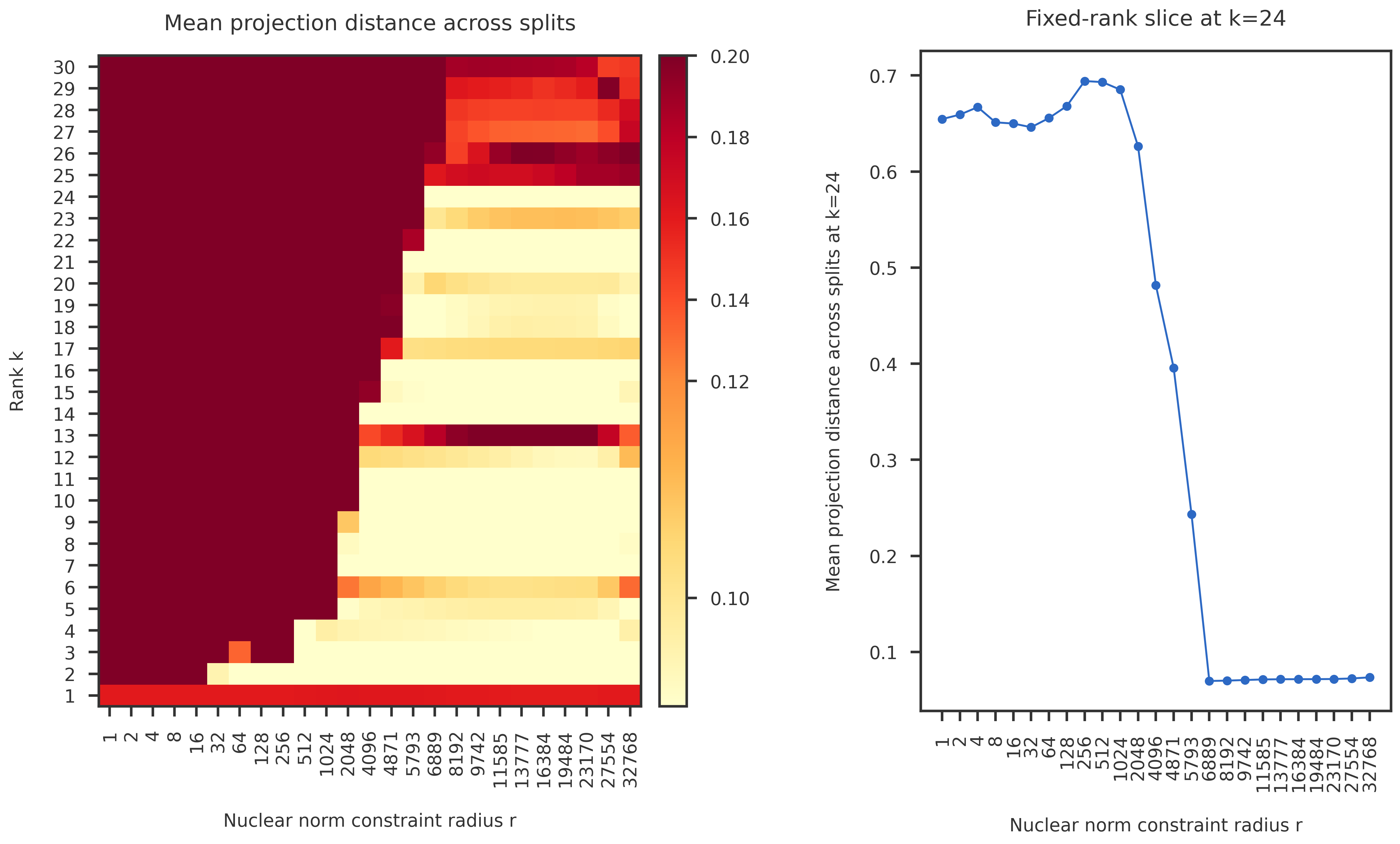
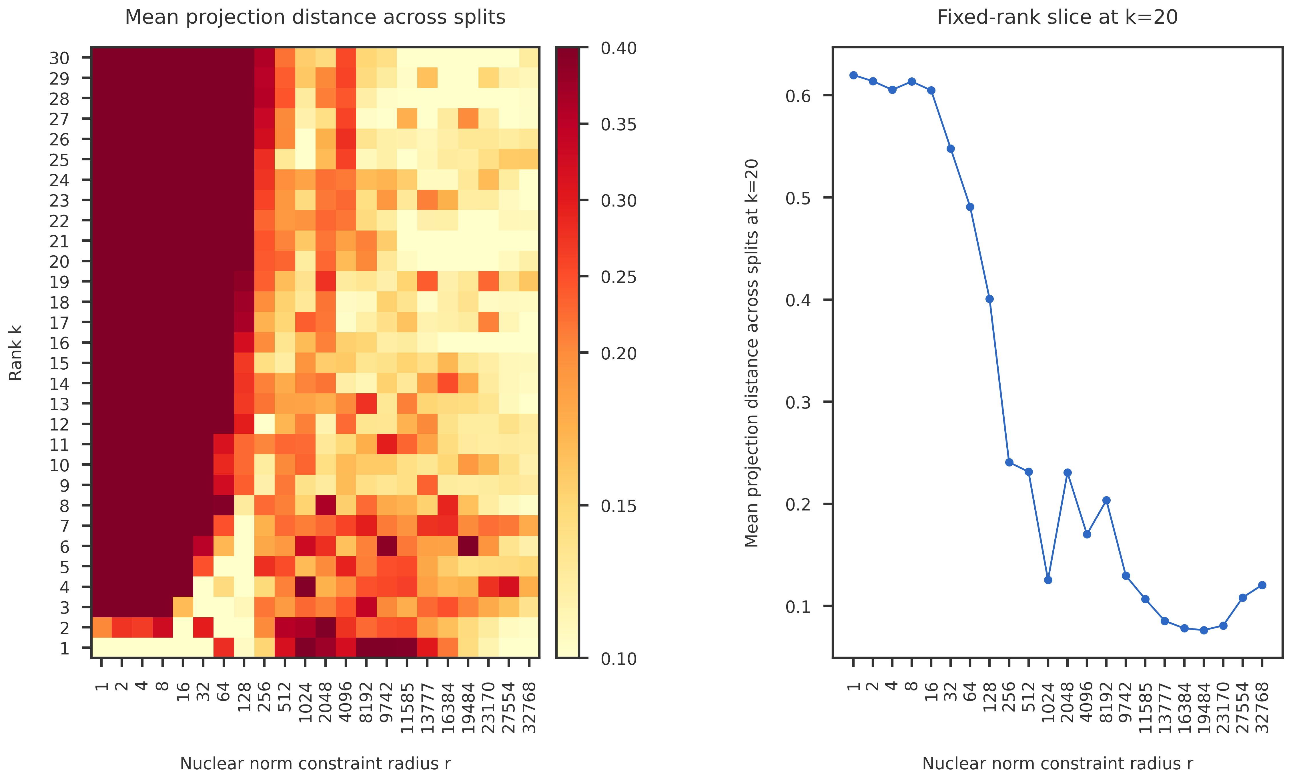
def make_projection_distance_figure(prefix,
        k_choose=24, vmin=0.09, vcenter=0.12, vmax=0.2):
    records = load_stability_jsons(stability_out_dir, prefix)
    dist_df = build_by_k_metrics_grid(records, "mean_dist", duplicate="first")
    rank_list = dist_df.columns.to_numpy()
    k_list = dist_df.index.to_numpy()
 
    fig = plt.figure(figsize=(15, 9), constrained_layout=True)
    gs = fig.add_gridspec(nrows=1, ncols=2, 
                          width_ratios=[1, 0.8],  # heatmap, line plot
                          wspace=0.2,
                         )
    ax1 = fig.add_subplot(gs[0, 0])
    ax2 = fig.add_subplot(gs[0, 1])

    plot_heatmap(ax1, dist_df.to_numpy(), rank_list, k_list, 
                 vmin=vmin, vcenter=vcenter, vmax=vmax)
    ax1.set_title("Mean projection distance across splits", pad = 20)

    # Plot a single row of the heatmap as a line plot. 
    # Makes it easier to see the plateau onset for one chosen rank.
    dist_vals = dist_df.loc[k_choose].to_numpy()
    ax2.plot(np.arange(len(dist_vals)), dist_vals, 'o-')
    ax2.set_xlabel("Nuclear norm constraint radius r")
    ax2.set_ylabel(f"Mean projection distance across splits at k={k_choose:d}")
    ax2.set_xticks(np.arange(len(dist_vals)))
    ax2.set_xticklabels(rank_list, rotation=90)
    ax2.set_title(f"Fixed-rank slice at k={k_choose}", pad = 20)
    
    fig.savefig(
        fig_dir / f"{prefix}_projection_distance.png",
        bbox_inches="tight",
    )
    plt.close(fig)
    # plt.show()
    

for prefix in PREFIXES:
    k_choose = 24
    vmin, vcenter, vmax = 0.09, 0.12, 0.20
    if prefix == "pgd_afw_nnm_corr":
        k_choose = 20
        vmin, vcenter, vmax = 0.1, 0.2, 0.4
    make_projection_distance_figure(prefix,
        k_choose=k_choose, vmin=vmin, vcenter=vcenter, vmax=vmax)

Diagnostics

These plots are secondary checks. They help distinguish a real stability plateau from artifacts caused by changing effective rank or unstable high-dimensional directions.

Code
def make_diagnostics_energy_angle_figure(prefix):
    records      = load_stability_jsons(stability_out_dir, prefix)
    energy_df    = build_by_k_metrics_grid(records, "mean_energy", duplicate="first")
    gap_angle_df = build_by_k_metrics_grid(records, "mean_gap_angle", duplicate="first")
    rank_list = energy_df.columns.to_numpy()
    k_list = energy_df.index.to_numpy()

    fig = plt.figure(figsize=(15, 9), constrained_layout=True)
    gs = fig.add_gridspec(nrows=1, ncols=2, 
                          width_ratios=[1, 1],
                          wspace=0.2,
                         )
    ax1 = fig.add_subplot(gs[0, 0])
    ax2 = fig.add_subplot(gs[0, 1])

    plot_heatmap(ax1, energy_df.to_numpy(), rank_list, k_list, vmin = 0.8, vcenter = 0.9, vmax = 1.0)
    ax1.set_title("Mean cumulative singular-value energy", pad = 20)

    rank_list = gap_angle_df.columns.to_numpy()
    k_list = gap_angle_df.index.to_numpy()
    plot_heatmap(ax2, gap_angle_df.to_numpy(), rank_list, k_list, vmin = 0, vcenter = 45, vmax = 90.0)
    ax2.set_title("Mean largest principal angle across splits", pad = 20)
    
    fig.savefig(
        fig_dir / f"{prefix}_energy_gap_angle.png",
        bbox_inches="tight",
    )
    plt.close(fig)
    
for prefix in PREFIXES:
    make_diagnostics_energy_angle_figure(prefix)