ColormaNN manuscript figures - PanUKB T2D

Author

Saikat Banerjee

Published

April 10, 2025

Abstract

High quality plots used for PanUKB type 2 diabetes, using NYGC color palette.

Code

import numpy as np
import pandas as pd
import pickle
import sys
import os
import re

import matplotlib
import matplotlib.pyplot as plt
from pymir import mpl_stylesheet
from pymir import mpl_utils

import scipy.stats as sc_stats
import collections
import textalloc
from adjustText import adjust_text

# For OpenTargets API
import requests
import json

Code

# import matplotlib.font_manager as mpl_fm
# font_path = '/gpfs/commons/home/sbanerjee/nygc/Futura'
# mpl_fm.fontManager.addfont(font_path + '/FuturaStd-Book.otf') # Loads "Futura Std"

# mpl_stylesheet.banskt_presentation(splinecolor = 'black', dpi = 300)
# futura_book = FontProperties(fname='/gpfs/commons/home/sbanerjee/nygc/Futura/FuturaStd-Book.otf')

# NYGC Color Palette
nygc_colors = {
    'brown': '#7F0814',
    'darkred': '#d42e12',
    'orange': '#F37239',
    'darkyellow': '#F79320',
    'yellow': '#FFE438',
    'darkblue': '#003059',
    'blue': '#266DB6',
    'lightblue': '#A3D5ED',
    'darkgreen': '#006838',
    'green': '#0A8A42',
    'lightgreen': '#74B74A',
    'yellowgreen': '#BAD75F',
    'darkgray': '#1A1A1A',
    'gray': '#666666',
    'lightgray': '#CCCCCC',
    'khaki': '#ADA194',
    'darkkhaki': '#5E514D',
}

# Style sheet for manuscript
mpl_stylesheet.banskt_presentation(dpi = 300, fontsize = 18, 
    splinecolor = nygc_colors['darkgray'], black = nygc_colors['darkgray'])
# plt.rcParams['font.family'] = 'Futura Std'

Code

def iqr_outlier(x, axis = None, bar = 1.5, side = 'both'):
    assert side in ['gt', 'lt', 'both'], 'Side should be `gt`, `lt` or `both`.'
    
    def q1(x, axis = None):
        return np.percentile(x, 25, axis = axis)

    def q3(x, axis = None):
        return np.percentile(x, 75, axis = axis)

    d_iqr = sc_stats.iqr(x, axis = axis)
    d_q1 = q1(x, axis = axis)
    d_q3 = q3(x, axis = axis)
    iqr_distance = np.multiply(d_iqr, bar)

    stat_shape = list(x.shape)

    if isinstance(axis, collections.abc.Iterable):
        for single_axis in axis:
            stat_shape[single_axis] = 1
    else:
        stat_shape[axis] = 1

    if side in ['gt', 'both']:
        upper_range = d_q3 + iqr_distance
        upper_outlier = np.greater(x - upper_range.reshape(stat_shape), 0)
    if side in ['lt', 'both']:
        lower_range = d_q1 - iqr_distance
        lower_outlier = np.less(x - lower_range.reshape(stat_shape), 0)

    if side == 'gt':
        return upper_outlier
    if side == 'lt':
        return lower_outlier
    if side == 'both':
        return np.logical_or(upper_outlier, lower_outlier)

Code

data_dir = "/gpfs/commons/home/sbanerjee/work/npd/PanUKB/data"
result_dir = "/gpfs/commons/home/sbanerjee/npddata/panukb/results/colormann-svd"

zscore_df = pd.read_pickle(os.path.join(data_dir, f"modselect/zscore_noRx.pkl"))
trait_df  = pd.read_pickle(os.path.join(data_dir, f"modselect/traits_all_with_desc.pkl"))

variant_filename = f"{data_dir}/allvar.pruned.closesttss.hugo"
variant_df = pd.read_csv(variant_filename, sep = '\t')

nsample_filename = "/gpfs/commons/home/sbanerjee/work/npd/PanUKB/data/phe2483.SampleN.tsv"
nsample_df = pd.read_csv(nsample_filename, sep = '\t')

Code

methods = ["nnm", "nnm-sparse", "rpca"]
method_names = {
    "nnm" : "NNM",
    "nnm-sparse" : "NNM-Sparse",
    "rpca" : "Robust PCA"
}

res_pklfile = {
    "nnm": "nnm_model_r155872_iter1000.pkl",
    "nnm-sparse": "nnm_sparse_model_r155872_iter1000.pkl",
    "rpca": "rpca_model.pkl"
}

pca_comps = dict()
mf_comps = dict()
k = 200

for method in methods:
    comps_filename = os.path.join(result_dir, method, "noRx", "pca_comps.pkl")
    with open(comps_filename, "rb") as mfile:
        pca_comps[method] = pickle.load(mfile)
    mf_comps_filename = os.path.join(result_dir, method, "noRx", f"mf_comps_k{k}.pkl")
    with open(mf_comps_filename, "rb") as mfile:
        mf_comps[method] = pickle.load(mfile)
        
X = np.array(zscore_df.values.T)
X_cent = X - np.mean(X, axis = 0, keepdims = True)

Code

pheno_zindex = [int(x[1:]) for x in zscore_df.columns]
trait_df_noRx = trait_df.loc[trait_df['zindex'].isin(pheno_zindex)]
nsample_df_noRx = nsample_df.loc[trait_df_noRx.index]
trait_df_noRx.info()

<class 'pandas.core.frame.DataFrame'>
Index: 2110 entries, 0 to 2482
Data columns (total 20 columns):
 #   Column                       Non-Null Count  Dtype  
---  ------                       --------------  -----  
 0   zindex                       2110 non-null   int64  
 1   trait_type                   2110 non-null   object 
 2   phenocode                    2110 non-null   object 
 3   pheno_sex                    2110 non-null   object 
 4   coding                       267 non-null    object 
 5   modifier                     394 non-null    object 
 6   description                  2110 non-null   object 
 7   description_more             1408 non-null   object 
 8   coding_description           261 non-null    object 
 9   category                     2072 non-null   object 
 10  BIN_QT                       2110 non-null   object 
 11  n_cases_EUR                  2110 non-null   int64  
 12  n_controls_EUR               1304 non-null   float64
 13  N                            2110 non-null   int64  
 14  Neff                         2110 non-null   float64
 15  filename                     2110 non-null   object 
 16  aws_link                     2110 non-null   object 
 17  estimates.final.h2_observed  2106 non-null   float64
 18  long_description             2110 non-null   object 
 19  short_description            2110 non-null   object 
dtypes: float64(3), int64(3), object(14)
memory usage: 346.2+ KB

Code

focal_disease = {
    "opentarget_name" : "type 1 diabetes mellitus",
    "opentarget_id": "MONDO_0005147",
    "df_query_string": "Type 1 diabetes",
}

focal_disease = {
    "opentarget_name" : "type 2 diabetes mellitus",
    "opentarget_id": "MONDO_0005148",
    "df_query_string": "Type 2 diabetes",
}

trait_df_noRx.query(f"description == '{focal_disease['df_query_string']}'")

	zindex	trait_type	phenocode	pheno_sex	coding	modifier	description	description_more	coding_description	category	BIN_QT	n_cases_EUR	n_controls_EUR	N	Neff	filename	aws_link	estimates.final.h2_observed	long_description	short_description
459	460	phecode	250.2	both_sexes	NaN	NaN	Type 2 diabetes	NaN	NaN	endocrine/metabolic	BIN	22768	396181.0	418949	43061.32254	phecode-250.2-both_sexes.tsv.bgz	https://pan-ukb-us-east-1.s3.amazonaws.com/sum...	0.0484	Type 2 diabetes	Type 2 diabetes

Code

zindex = trait_df_noRx.query(f"description == '{focal_disease['df_query_string']}'")["zindex"].values[0]
method = "rpca"

trait_indices = np.array(trait_df_noRx.index)
tidx = np.searchsorted(trait_indices, zindex - 1)

loadings, factors, cos2_pheno, cos2_variant, contribution_pheno, contribution_variant = mf_comps[method]

Code

def get_opentarget_score(gene_id):

    # Build query string to get association information
    query_string = """
        query TargetAssociationsQuery(
          $ensemblId: String!
          $filter: String
          $sortBy: String!
          $enableIndirect: Boolean!
        ) {
          target(ensemblId: $ensemblId) {
            id
            approvedSymbol
            associatedDiseases(
              orderByScore: $sortBy
              BFilter: $filter
              enableIndirect: $enableIndirect
            ) {
              count
              rows {
                disease {
                  id
                  name
                }
                score
              }
            }
          }
        }

    """

    # Set variables object of arguments to be passed to endpoint
    variables = {
        "ensemblId": gene_id, 
        "filter": focal_disease["opentarget_name"],
        "sortBy": "score",
        "enableIndirect": False
    }

    # Set base URL of GraphQL API endpoint
    base_url = "https://api.platform.opentargets.org/api/v4/graphql"
    # print (gene_id)

    # Perform POST request and check status code of response
    r = requests.post(base_url, json={"query": query_string, "variables": variables})
    # print(r.status_code)

    # Transform API response from JSON into Python dictionary and print in console
    api_response = json.loads(r.text)
    # print(api_response)

    score = 0.0
    if api_response['data']['target'] is not None:
        associated_diseases = api_response['data']['target']['associatedDiseases']['rows']
        for d in associated_diseases:
            if d['disease']['id'] == focal_disease["opentarget_id"]:
                score = d['score']
    # print(score)
    return score

def get_variant_names(df):
    vstr_list = list()
    for i in range(df.shape[0]):
        vstr = 'chr' + df.iloc[i][['chr', 'rsid', 'Gene_name']].astype('str').str.cat(sep=' | ')
        gene_id = df.iloc[i]['ensembl_gene_id']
        if not pd.isna(gene_id):
            assoc_score = get_opentarget_score(gene_id)
            vstr += f" | {assoc_score:.3f}"
        else:
            vstr += f" | NaN"
        vstr_list.append(vstr)
    return vstr_list

Code

top_factor1 = np.argsort(cos2_pheno[tidx,:])[::-1][0]
top_factor2 = np.argsort(cos2_pheno[tidx,:])[::-1][1]
top_factor3 = np.argsort(cos2_pheno[tidx,:])[::-1][2]
top_factor4 = np.argsort(cos2_pheno[tidx,:])[::-1][3]

Code

np.sort(cos2_pheno[tidx,:])[::-1][:4]

array([0.16283928, 0.15683106, 0.07770912, 0.05925545])

Code

n_plot_variants = 20

top_variant_idx = np.argsort(contribution_variant[:, top_factor1])[::-1][:n_plot_variants]
top_variant_df = variant_df.loc[zscore_df.index.to_numpy()[top_variant_idx]]
top_variant_score = contribution_variant[top_variant_idx, top_factor1]   
top_variant_names = get_variant_names(top_variant_df)

Code

cts_resdir = "/gpfs/commons/home/sbanerjee/npddata/panukb/results/ldsc"
cts_resfile = os.path.join(cts_resdir, method, "enrich", f"factor_{top_factor1}_sumstat.Multi_tissue_gene_expr.cell_type_results.txt")
n_plot_tissues = 10

cts_df = pd.read_csv(cts_resfile, sep="\t").sort_values(by=["Coefficient_P_value"]).head(n_plot_tissues)
cts_df

	Name	Coefficient	Coefficient_std_error	Coefficient_P_value
130	A09.371.729.Retina	5.559657e-08	2.473752e-08	0.012305
26	Liver	5.741948e-08	2.674653e-08	0.015905
104	A05.810.453.Kidney	4.497565e-08	2.257740e-08	0.023182
0	Adrenal_Gland	5.095011e-08	2.640198e-08	0.026817
52	A02.835.232.834.151.Cervical.Vertebrae	4.938831e-08	2.668004e-08	0.032075
182	A11.872.700.500.Induced.Pluripotent.Stem.Cells	5.117475e-08	2.801075e-08	0.033852
183	A11.872.190.Embryonic.Stem.Cells	4.902852e-08	2.710032e-08	0.035214
156	A11.329.114.Adipocytes	4.277042e-08	2.432691e-08	0.039361
157	A08.186.211.865.428.Metencephalon	3.531917e-08	2.016059e-08	0.039896
1	Brain_Cerebellum	3.663629e-08	2.101926e-08	0.040668

Code

# cts_df["Name"] = ["Pancreas", "Liver", "Ileum", "Breast Mammary Tissue", "Intestinal Mucosa",
#                         "Kidney", "Subcutaneous Fat", "Embryonic Stem Cells", 
#                         "Small Intestine Terminal Ileum", "Kidney Cortex"]
cts_df["Name"] = ["Retina", "Liver", "Kidney", "Adrenal Gland", "Cervical Vertebrae",
                        "IPSC", "Embryonic Stem Cells", "Adipocytes", 
                        "Metencephalon", "Kidney Cortex"]
cts_df

	Name	Coefficient	Coefficient_std_error	Coefficient_P_value
130	Retina	5.559657e-08	2.473752e-08	0.012305
26	Liver	5.741948e-08	2.674653e-08	0.015905
104	Kidney	4.497565e-08	2.257740e-08	0.023182
0	Adrenal Gland	5.095011e-08	2.640198e-08	0.026817
52	Cervical Vertebrae	4.938831e-08	2.668004e-08	0.032075
182	IPSC	5.117475e-08	2.801075e-08	0.033852
183	Embryonic Stem Cells	4.902852e-08	2.710032e-08	0.035214
156	Adipocytes	4.277042e-08	2.432691e-08	0.039361
157	Metencephalon	3.531917e-08	2.016059e-08	0.039896
1	Kidney Cortex	3.663629e-08	2.101926e-08	0.040668

Code

import matplotlib.gridspec as gridspec
fig = plt.figure(figsize = (22, 22))

gs = fig.add_gridspec(2, 2, height_ratios=(1, 1), width_ratios = (2,1), wspace=0, hspace=0)

ax1 = fig.add_subplot(gs[0,0])
ax2 = fig.add_subplot(gs[1,0])

gs_rcol = gridspec.GridSpecFromSubplotSpec(2, 1, subplot_spec=gs[0:2,1], height_ratios = (2, 1))
axr1 = fig.add_subplot(gs_rcol[0, 0])
axr2 = fig.add_subplot(gs_rcol[1, 0])

# PC1 vs PC2
xvals = - loadings[:, top_factor2]
yvals = - loadings[:, top_factor3]

# Combine outliers in x-axis and y-axis
# outlier_idx_x = np.where(iqr_outlier(xvals, axis = 0, bar = 5.0))[0]
# outlier_idx_y = np.where(iqr_outlier(yvals, axis = 0, bar = 5.0))[0]
outlier_idx_x = np.argsort(contribution_pheno[:, top_factor2])[::-1][:20]
outlier_idx_y = np.argsort(contribution_pheno[:, top_factor3])[::-1][:40]
outlier_idx = np.union1d(outlier_idx_x, outlier_idx_y)
x_center = np.mean(ax1.get_xlim())
common_idx = np.setdiff1d(np.arange(xvals.shape[0]), outlier_idx)
txt_list = []
text_idx_list = []
for i in outlier_idx:
    if i != tidx:
        txt = trait_df_noRx.loc[trait_indices[i]]['short_description'].strip()
        txt_list.append(txt)
        text_idx_list.append(i)
# Mark Type 2 diabetes
txt_list.append("Type 2 Diabetes")
text_idx_list.append(tidx)

scatter_plot = ax1.scatter(xvals[outlier_idx], yvals[outlier_idx], alpha = 0.7, s = 100, color = nygc_colors['orange'])
ax1.scatter(xvals[tidx], yvals[tidx], s = 150, color = nygc_colors['blue'])
ax1.scatter(xvals[common_idx], yvals[common_idx], alpha = 0.1, s = 100, color = nygc_colors['khaki'])

# # Mark using textalloc package
if len(text_idx_list) > 0:
    txt_idx = np.array(text_idx_list)
    textalloc.allocate_text(fig, ax1, xvals[txt_idx], yvals[txt_idx], txt_list,
                            # x_scatter = xvals, y_scatter = yvals,
                            scatter_plot = scatter_plot,
                            textsize = 10, textcolor = 'black', linecolor = nygc_colors['gray'])

# # Mark using adjustText package
# # https://github.com/Phlya/adjustText
# annots = []
# for i, txt in zip(text_idx_list, txt_list):
#     if xvals[i] > x_center:
#         annots += [ax1.annotate(txt, (xvals[i], yvals[i]), fontsize = 6, ha = 'right')]
#     else:
#         annots += [ax1.annotate(txt, (xvals[i], yvals[i]), fontsize = 6)]
# adjust_text(annots, arrowprops=dict(arrowstyle='-', color = nygc_colors['gray']))


# ax1.set_xticks([-0.010, -0.005, 0.0, 0.005, 0.010])
for side, border in ax1.spines.items():
    if side == 'left':
        border.set_bounds(-0.06, 0.04)
    elif side == 'bottom':
        border.set_bounds(-0.05, 0.03)
    else:
        border.set_visible(False)
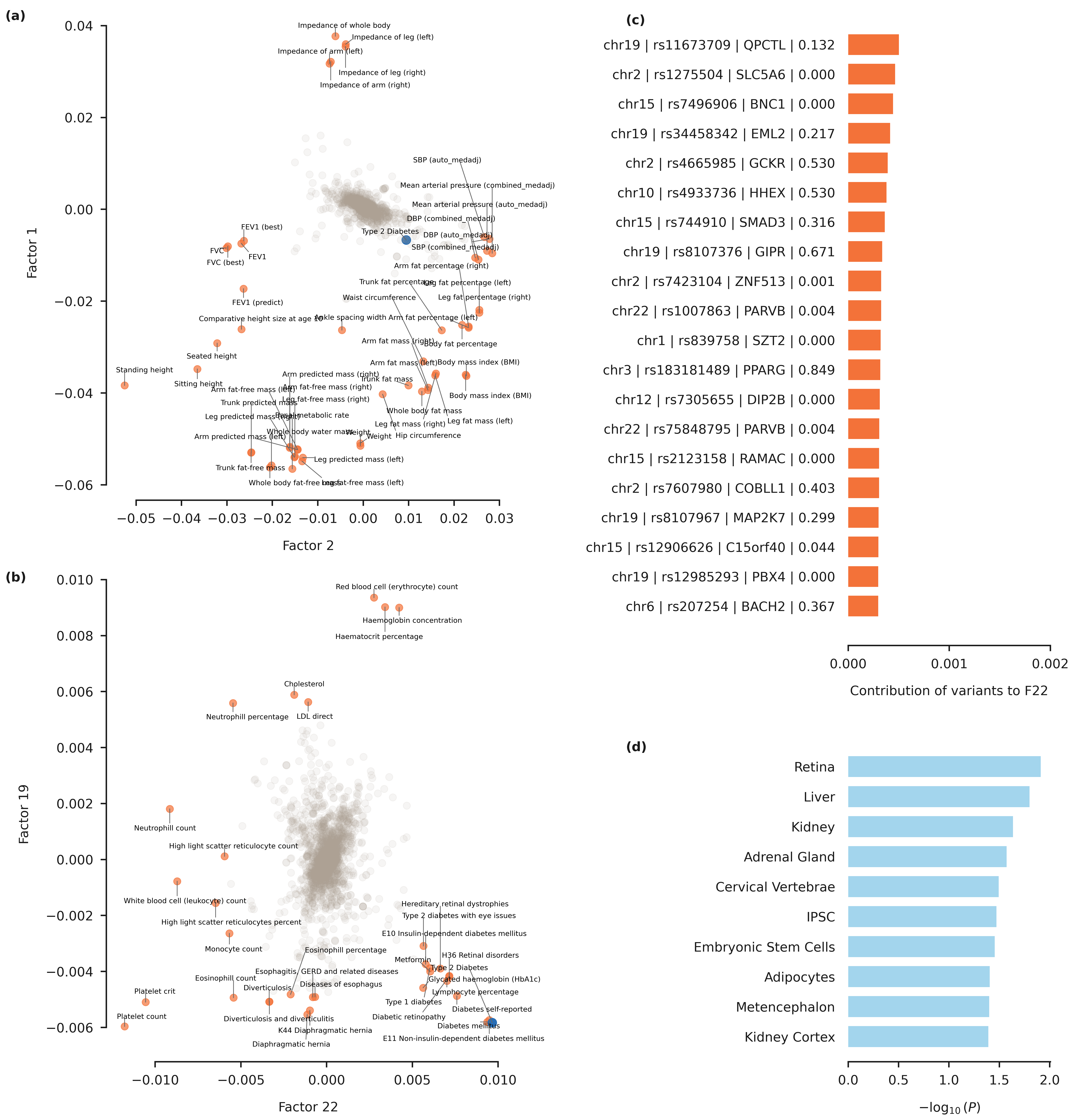
ax1.set_xlabel(f"Factor {top_factor2 + 1}")
ax1.set_ylabel(f"Factor {top_factor3 + 1}")

# PC22 vs PC19 on ax2
xvals = loadings[:, top_factor1]
yvals = - loadings[:, top_factor4]

# Combine outliers in x-axis and y-axis
# outlier_idx_x = np.where(iqr_outlier(xvals, axis = 0, bar = 5.0))[0]
# outlier_idx_y = np.where(iqr_outlier(yvals, axis = 0, bar = 5.0))[0]
outlier_idx_x = np.argsort(contribution_pheno[:, top_factor1])[::-1][:20]
outlier_idx_y = np.argsort(contribution_pheno[:, top_factor4])[::-1][:20]
outlier_idx = np.union1d(outlier_idx_x, outlier_idx_y)
x_center = np.mean(ax2.get_xlim())
common_idx = np.setdiff1d(np.arange(xvals.shape[0]), outlier_idx)
txt_list = []
text_idx_list = []
for i in outlier_idx:
    if i != tidx:
        txt = trait_df_noRx.loc[trait_indices[i]]['short_description'].strip()
        txt_list.append(txt)
        text_idx_list.append(i)
# Mark Type 2 diabetes
txt_list.append("Type 2 Diabetes")
text_idx_list.append(tidx)

scatter_plot = ax2.scatter(xvals[outlier_idx], yvals[outlier_idx], alpha = 0.7, s = 100, color = nygc_colors['orange'])
ax2.scatter(xvals[tidx], yvals[tidx], s = 150, color = nygc_colors['blue'])
ax2.scatter(xvals[common_idx], yvals[common_idx], alpha = 0.1, s = 100, color = nygc_colors['khaki'])

# # Mark using textalloc package
if len(text_idx_list) > 0:
    txt_idx = np.array(text_idx_list)
    textalloc.allocate_text(fig, ax2, xvals[txt_idx], yvals[txt_idx], txt_list,
                            # x_scatter = xvals, y_scatter = yvals,
                            scatter_plot = scatter_plot,
                            textsize = 10, textcolor = 'black', linecolor = nygc_colors['gray'])

# ax1.set_xticks([-0.010, -0.005, 0.0, 0.005, 0.010])
for side, border in ax2.spines.items():
    if side == 'left':
        border.set_bounds(-0.006, 0.01)
    elif side == 'bottom':
        border.set_bounds(-0.01, 0.01)
    else:
        border.set_visible(False)
ax2.set_xlabel(f"Factor {top_factor1 + 1}")
ax2.set_ylabel(f"Factor {top_factor4 + 1}")

# Contribution of variants
xvals = top_variant_score
yvals = np.arange(n_plot_variants)[::-1]

axr1.barh(yvals, xvals, align = 'center', height = 0.7, color = nygc_colors['orange'], edgecolor = 'None')
axr1.set_yticks(yvals)
axr1.set_yticklabels(top_variant_names)

for side in ['top', 'right', 'left']:
    axr1.spines[side].set_visible(False)

axr1.tick_params(left=False)
axr1.set_xlabel(f"Contribution of variants to F{top_factor1 + 1}")
axr1.set_xticks([0, 0.001, 0.002])
# ax1.set_title(method_names[method])

# Enrichment
xvals = -np.log10(cts_df["Coefficient_P_value"].to_numpy())
yvals = np.arange(n_plot_tissues)[::-1]

axr2.barh(yvals, xvals, align = 'center', height = 0.7, color = nygc_colors['lightblue'], edgecolor = 'None')
axr2.set_yticks(yvals)
axr2.set_yticklabels(cts_df["Name"])

for side in ['top', 'right', 'left']:
    axr2.spines[side].set_visible(False)

axr2.tick_params(left=False)
axr2.set_xlabel(r"$-\log_{10}(P)$")

# Panel labels
ax1.text(-0.25, 0.97, "(a)", transform=ax1.transAxes, fontweight='bold')
ax2.text(-0.25, 0.97, "(b)", transform=ax2.transAxes, fontweight='bold')
axr1.text(-1.10, 0.97, "(c)", transform=axr1.transAxes, fontweight='bold')
axr2.text(-1.10, 0.97, "(d)", transform=axr2.transAxes, fontweight='bold')

gs.tight_layout(fig)
plt.savefig('../plots/colormann-manuscript/panukb_t2d_rpca.pdf', bbox_inches='tight')
plt.show()

Code

fig = plt.figure(figsize = (12, 6))
ax1 = fig.add_subplot(121)
ax2 = fig.add_subplot(122)

xvals = np.arange(cos2_pheno[tidx,:].shape[0])
yvals = cos2_pheno[tidx,:]
ax1.bar(xvals, yvals, align = 'center', width = 0.1)

xvals = np.arange(contribution_pheno[tidx, :].shape[0])
yvals = contribution_pheno[tidx, :]
ax2.bar(xvals, yvals, align = 'center', width = 0.05)

for side in ['top', 'right']:
    ax1.spines[side].set_visible(False)
    ax2.spines[side].set_visible(False)
    
ax1.tick_params(bottom=False)
ax1.set_ylabel(f"Importance ($\cos^2$ score)")
ax1.set_xlabel(f"Factors")

ax2.tick_params(bottom=False)
ax2.set_ylabel(f"T2D contribution")
ax2.set_xlabel(f"Factors")

plt.tight_layout()
plt.savefig('../plots/colormann-manuscript/panukb_t2d_rpca_cos2_contr.pdf', bbox_inches='tight')
plt.show()