Comparison of different methods using numerical experiments

Author

Saikat Banerjee

Published

December 29, 2023

Abstract

We perform numerical experiments to compare the power and efficiency of different methods in detecting the hidden genetics factors contributing to disease pleiotropy.

Getting Setup

Code

import numpy as np
import pandas as pd
import pickle
import sys
import os
import dsc
from dsc.query_engine import Query_Processor as dscQP
from dsc import dsc_io

import matplotlib.pyplot as plt
from pymir import mpl_stylesheet
from pymir import mpl_utils
mpl_stylesheet.banskt_presentation(splinecolor = 'black', dpi = 120)

Code

def stratify_dfcol(df, colname, value):
    #return pd_utils.select_dfrows(df, [f"$({colname}) == {value}"])
    return df.loc[df[colname] == value]

def stratify_dfcols(df, condition_list):
    for (colname, value) in condition_list:
        df = stratify_dfcol(df, colname, value)
    return df

def stratify_dfcols_in_list(df, colname, values):
    return df.loc[df[colname].isin(values)]

Read Simulation Results

Code

dsc_output = "/gpfs/commons/groups/knowles_lab/sbanerjee/low_rank_matrix_approximation_numerical_experiments/blockdiag"
dsc_fname  = os.path.basename(os.path.normpath(dsc_output))
db = os.path.join(dsc_output, dsc_fname + ".db")
dscoutpkl = os.path.join("/gpfs/commons/home/sbanerjee/work/npd/lrma-dsc/dsc/results", dsc_fname + "_dscout.pkl")
dscout    = pd.read_pickle(dscoutpkl)
dscout

	DSC	simulate	simulate.n	simulate.p	simulate.k	simulate.h2	simulate.h2_shared_frac	simulate.aq	lowrankfit	matfactor	score.L_rmse	score.F_rmse	score.Z_rmse	score.L_psnr	score.F_psnr	score.Z_psnr	score.adj_MI
0	1	blockdiag	200.0	2000.0	10.0	0.2	0.5	0.6	identical	truncated_svd	0.244982	0.485097	0.005098	28.429593	24.712971	21.552452	0.018100
1	2	blockdiag	200.0	2000.0	10.0	0.2	0.5	0.6	identical	truncated_svd	0.264152	0.483567	0.005141	28.688465	24.252872	21.767697	0.015638
2	3	blockdiag	200.0	2000.0	10.0	0.2	0.5	0.6	identical	truncated_svd	0.252526	0.499034	0.005091	28.831802	23.687408	22.263407	0.654857
3	4	blockdiag	200.0	2000.0	10.0	0.2	0.5	0.6	identical	truncated_svd	0.285154	0.484862	0.005550	28.881899	24.282865	23.215231	0.561981
4	5	blockdiag	200.0	2000.0	10.0	0.2	0.5	0.6	identical	truncated_svd	0.292962	0.474069	0.005080	27.246965	24.492696	22.070442	0.024386
...	...	...	...	...	...	...	...	...	...	...	...	...	...	...	...	...	...
895	8	blockdiag_aq	200.0	2000.0	10.0	0.2	0.5	0.8	identical	factorgo	0.597619	0.720961	0.002017	20.790216	21.536737	30.477673	0.010297
896	9	blockdiag_aq	200.0	2000.0	10.0	0.2	0.5	0.4	identical	factorgo	0.201241	0.400942	0.002174	30.378105	26.809769	29.938074	-0.009727
897	9	blockdiag_aq	200.0	2000.0	10.0	0.2	0.5	0.8	identical	factorgo	0.509286	0.669955	0.002038	21.469111	20.631187	28.405981	0.003175
898	10	blockdiag_aq	200.0	2000.0	10.0	0.2	0.5	0.4	identical	factorgo	0.270847	0.429577	0.002189	28.086705	25.500348	30.518931	0.022548
899	10	blockdiag_aq	200.0	2000.0	10.0	0.2	0.5	0.8	identical	factorgo	0.626669	0.756680	0.002087	19.320562	20.277492	30.701310	-0.004610

900 rows × 17 columns

Compare Methods

We use several metrics to compare the different methods.

methods = {
    "rpca" : ["rpca", "truncated_svd"],
    "nnm"  : ["nnm", "truncated_svd"],
    "nnm_sparse" : ["nnm_sparse", "truncated_svd"],
    "truncated_svd" : ["identical", "truncated_svd"],
    "factorgo" : ["identical", "factorgo"],
}
method_labels = {
    "rpca" : "RPCA-IALM",
    "nnm" : "NN-FW",
    "nnm_sparse" : "NN-Sparse-FW",
    "truncated_svd": "tSVD",
    "factorgo": "FactorGO",
}

method_colors = {
    "rpca" : '#FF6800', # Vivid Orange
    "nnm" : '#C10020', # Vivid Red
    "nnm_sparse" : '#803E75', # Strong Purple
    "truncated_svd" : '#535154', # gray
    "factorgo" : '#A6BDD7', # Very Light Blue
}

# Base parameters
simparams = {'p': 2000, 'k': 10, 'h2': 0.2, 'h2_shared_frac': 0.5, 'aq': 0.6}
score_names = {
    'L_rmse': r"$\| L - \hat{L}\|_F$",
    'F_rmse': r"$\| F - \hat{F}\|_F$",
    'Z_rmse': r"$\| LF^{T} - \hat{L}\hat{F}^{T}\|_F$",
    'adj_MI': "Adjusted Mutual Information Score",
}

# score_names = {
#     'L_psnr': r"$\| L - \hat{L}\|_F$",
#     'F_psnr': r"$\| F - \hat{F}\|_F$",
#     'Z_psnr': r"$\| LF^{T} - \hat{L}\hat{F}^{T}\|_F$",
#     'adj_MI': "Adjusted Mutual Information Score",
# }

Code

def get_simulation_with_variable(df, var_name, var_values):
    condition = [(f'simulate.{k}', v) for k, v in simparams.items() if k != var_name]
    df1 = stratify_dfcols(df, condition)
    df2 = stratify_dfcols_in_list(df1, f'simulate.{var_name}', var_values)
    return df2

def get_scores_from_dataframe(df, score_name, variable_name, variable_values, 
        methods = methods):
    simdf = get_simulation_with_variable(df, variable_name, variable_values)
    scores = {key: list() for key in methods.keys()}
    for method, mlist in methods.items():
        mrows = stratify_dfcols(simdf, [('lowrankfit', mlist[0]), ('matfactor', mlist[1])])
        for value in variable_values:
            vrows = stratify_dfcol(mrows, f'simulate.{variable_name}', value)
            scores[method].append(vrows[f'score.{score_name}'].to_numpy())
    return scores

Code

def random_jitter(xvals, yvals, d = 0.1):
    xjitter = [x + np.random.randn(len(y)) * d for x, y in zip(xvals, yvals)]
    return xjitter

def boxplot_scores(variable, variable_values, 
        methods = methods, score_names = score_names,
        dscout = dscout, method_colors = method_colors):
    
    nmethods = len(methods)
    nvariables = len(variable_values)
    nscores = len(score_names)
    
    figh = 6
    figw = (nscores * figh) + (nscores - 1)
    fig = plt.figure(figsize = (figw, figh))
    axs = [fig.add_subplot(1, nscores, x+1) for x in range(nscores)]
    boxs = {x: None for x in methods.keys()}
    
    for i, (score_name, score_label) in enumerate(score_names.items()):
        scores = get_scores_from_dataframe(dscout, score_name, variable, variable_values)
        for j, mkey in enumerate(methods.keys()):
            boxcolor = method_colors[mkey]
            boxface = f'#{boxcolor[1:]}80'
            medianprops = dict(linewidth=0, color = boxcolor)
            whiskerprops = dict(linewidth=2, color = boxcolor)
            boxprops = dict(linewidth=2, color = boxcolor, facecolor = boxface)
            flierprops = dict(marker='o', markerfacecolor=boxface, markersize=3, markeredgecolor = boxcolor)

            xpos = [x * (nmethods + 1) + j for x in range(nvariables)]
            boxs[mkey] = axs[i].boxplot(scores[mkey], positions = xpos,
                showcaps = False, showfliers = False,
                widths = 0.7, patch_artist = True, notch = False,
                flierprops = flierprops, boxprops = boxprops,
                medianprops = medianprops, whiskerprops = whiskerprops)
            
            axs[i].scatter(random_jitter(xpos, scores[mkey]), scores[mkey], 
                           edgecolor = boxcolor, facecolor = boxface, linewidths = 1, 
                           s = 10)

        xcenter = [x * (nmethods + 1) + (nmethods - 1) / 2 for x in range(nvariables)]
        axs[i].set_xticks(xcenter)
        axs[i].set_xticklabels(variable_values)
        axs[i].set_xlabel(variable)
        axs[i].set_ylabel(score_label)
        xlim_low = 0 - (nvariables - 1) / 2
        #xlim_high = (nvariables - 1) * (nmethods + 1) + (nmethods - 1) + (nvariables - 1) / 2
        xlim_high = (nmethods + 1.5) * nvariables - 2.5
        axs[i].set_xlim( xlim_low, xlim_high )

    plt.tight_layout()
    return axs, boxs

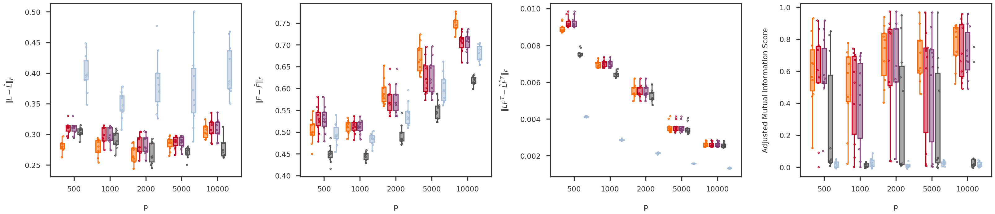
variable = 'p'
variable_values = [500, 1000, 2000, 5000, 10000]

axs, boxs = boxplot_scores(variable, variable_values)
plt.show()

Code

fig = plt.figure(figsize = (6, 2))
ax1 = fig.add_subplot(111)
handles = [boxs[mkey]["boxes"][0] for mkey in methods.keys()]
labels = [method_labels[mkey] for mkey in methods.keys()]
ax1.legend(handles = handles, labels = labels, loc = 'upper left', frameon = False, handlelength = 4, ncol = 2)

for side, border in ax1.spines.items():
    border.set_visible(False)
ax1.tick_params(bottom = False, top = False, left = False, right = False,
                   labelbottom = False, labeltop = False, labelleft = False, labelright = False)


plt.show()

Code

variable = 'k'
variable_values = [2,5,10,15,20]
boxplot_scores(variable, variable_values)
plt.show()

Code

variable = 'h2'
variable_values = [0.05, 0.1, 0.2, 0.3, 0.4]
boxplot_scores(variable, variable_values)
plt.show()

Code

variable = 'h2_shared_frac'
variable_values = [0.2, 0.5, 0.8, 1.0]
boxplot_scores(variable, variable_values)
plt.show()

Code

variable = 'aq'
variable_values = [0.4, 0.6, 0.8]
boxplot_scores(variable, variable_values)
plt.show()

PSNR

Instead of the Frobenius norm, we can also use the Peak Signal-to-Noise Ratio (PSNR) for comparing the methods.

Code

psnr_score_names = {
    'L_psnr': r"PSNR ($L$)",
    'F_psnr': r"PSNR ($F$)",
    'Z_psnr': r"PSNR ($LF^T$)",
}

variable = 'p'
variable_values = [500, 1000, 2000, 5000, 10000]

axs, boxs = boxplot_scores(variable, variable_values, score_names = psnr_score_names)
plt.show()