Comparison of different noise models

Abstract

Denoising can be done either using Gaussian noise or sparse noise or both. Here, I compare the three noise models.

About

Our goal is to obtain a denoised, low-rank approximation of the input matrix. Such low-rank matrix can be obtained using different noise models:

1. Gaussian noise \min_{\mathbf{X}} \frac{1}{2}\left\lVert \mathbf{Y} - \mathbf{X} \right\rVert_{F}^2 \quad \textrm{s.t.} \quad \left\lVert \mathbf{X} \right\rVert_{*} \le r
2. Sparse noise \min_{\mathbf{X}, \mathbf{M}} \left\lVert \mathbf{X} \right\rVert_{*} + \lambda \left\lVert \mathbf{M} \right\rVert_{1} \quad \textrm{s.t.} \quad \mathbf{L} + \mathbf{M} = \mathbf{Y}
3. Gaussian + sparse \min_{\mathbf{X}} \frac{1}{2}\left\lVert \mathbf{Y} - \mathbf{X} - \mathbf{M} \right\rVert_{F}^2 \quad \textrm{s.t.} \quad \left\lVert \mathbf{X} \right\rVert_{*} \le r_L\,, \left\lVert \mathbf{M} \right\rVert_{1} \le r_M

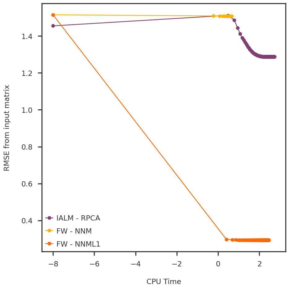
For models (1) and (3), we use the Frank-Wolfe method, and for model (2), we use the inexact augmented Lagrangian method (IALM) with a slight modification of the step-size update (borrowing the ADMM updates of Boyd et. al.). We use a simple simulation (as described previously) with additive Gaussian noise to realistically mimic the z-scores obtained from multiple GWAS.

Getting setup

We have now implemented a Python software to call the different methods with flexibility to choose different input options.

import numpy as np
import pandas as pd

import matplotlib.pyplot as plt
from pymir import mpl_stylesheet
from pymir import mpl_utils

mpl_stylesheet.banskt_presentation(splinecolor = 'black', dpi = 120, colors = 'kelly')import numpy as np
import pandas as pd

import matplotlib.pyplot as plt
from pymir import mpl_stylesheet
from pymir import mpl_utils

mpl_stylesheet.banskt_presentation(splinecolor = 'black', dpi = 120, colors = 'kelly')

import sys
sys.path.append("../utils/")
import histogram as mpy_histogram
import simulate as mpy_simulate
import plot_functions as mpy_plotfn

from nnwmf.optimize import IALM

import sys
sys.path.append("../utils/")
import histogram as mpy_histogram
import simulate as mpy_simulate
import plot_functions as mpy_plotfn

from nnwmf.optimize import IALM
from nnwmf.optimize import FrankWolfe
from nnwmf.utils import model_errors as merr

Simulation

ntrait = 4 # categories / class
ngwas  = 500 # N
nsnp   = 1000 # P
nfctr  = 40 # K

Y, Y_true, L, F, mean, noise_var, sample_indices = mpy_simulate.simulate(ngwas, nsnp, ntrait, nfctr, std = 1.5, do_shift_mean = False)
Y_cent = mpy_simulate.do_standardize(Y, scale = False)
Y_std  = mpy_simulate.do_standardize(Y)
Y_true_cent = mpy_simulate.do_standardize(Y_true, scale = False)

unique_labels  = list(range(len(sample_indices)))
class_labels = [None for x in range(ngwas)]
for k, idxs in enumerate(sample_indices):
    for i in idxs:
        class_labels[i] = k

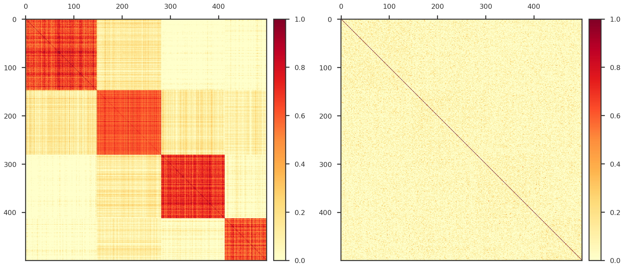
In Figure 1, we show the underlying structure of our simulated data. On the left panel, we show the covariance of the true loadings and on the right panel, we show the covariance of the observed data (strong noise removes the underlying correlation)

fig = plt.figure(figsize = (18, 8))
ax1 = fig.add_subplot(121)
ax2 = fig.add_subplot(122)

mpy_plotfn.plot_covariance_heatmap(ax1, L)
mpy_plotfn.plot_covariance_heatmap(ax2, Y)

plt.tight_layout(w_pad = 2.0)
plt.show()

Figure 1: Covariance structure of the true loadings in the simulation

Denoising Methods

We then apply the three methods.

IALM - RPCA

rpca = IALM(benchmark = True, max_iter = 1000, mu_update_method='admm', show_progress = True)
rpca.fit(Y_cent, Xtrue = Y_cent)

2023-08-02 14:46:55,016 | nnwmf.optimize.inexact_alm               | INFO    | Iteration 0. Primal residual 0.807755. Dual residual 0.00319521
2023-08-02 14:47:16,524 | nnwmf.optimize.inexact_alm               | INFO    | Iteration 100. Primal residual 6.9408e-06. Dual residual 1.68576e-06

FW - NNM

We do a little cheating here. Instead of cross-validation, we directly use the known rank of the underlying true data. However, based on my previous work, I know that cross-validation does provide the correct rank.

nnm = FrankWolfe(model = 'nnm', svd_max_iter = 50, 
                 show_progress = True, debug = True, benchmark = True)
nnm.fit(Y_cent, 40.0, Ytrue = Y_cent)

2023-08-02 14:47:37,144 | nnwmf.optimize.frankwolfe                | INFO    | Iteration 0. Step size 1.000. Duality Gap 5383.02

FW - NNML1

For the third model, we use the sparse noise threshold from the RPCA result and the rank from the true data. I have not checked cross-validation results for this method yet.

np.sum(np.abs(rpca.E_)) / (ngwas * nsnp)

0.7012888342395619

nnm_sparse = FrankWolfe(model = 'nnm-sparse', max_iter = 1000, svd_max_iter = 50, 
                        tol = 1e-3, step_tol = 1e-5, simplex_method = 'sort',
                        show_progress = True, debug = True, benchmark = True, print_skip = 100)
nnm_sparse.fit(Y_cent, (40.0, 0.7), Ytrue = Y_cent)

2023-08-02 14:47:49,393 | nnwmf.optimize.frankwolfe                | INFO    | Iteration 0. Step size 1.000. Duality Gap 6.42438e+06
2023-08-02 14:48:03,988 | nnwmf.optimize.frankwolfe                | INFO    | Iteration 100. Step size 0.004. Duality Gap 6.28097

Results

CPU time and accuracy

In Figure 2, we look at the RMSE (w.r.t the observed input data) and CPU time.

fig = plt.figure(figsize = (8, 8))
ax1 = fig.add_subplot(111)

kp = 0
ax1.plot(np.log10(np.cumsum(rpca.cpu_time_[kp:])), rpca.rmse_[kp:], 'o-', label = 'IALM - RPCA')
ax1.plot(np.log10(np.cumsum(nnm.cpu_time_[kp:])), nnm.rmse_[kp:], 'o-', label = 'FW - NNM')
ax1.plot(np.log10(np.cumsum(nnm_sparse.cpu_time_[kp:])), nnm_sparse.rmse_[kp:], 'o-', label = 'FW - NNML1')
ax1.legend()

ax1.set_xlabel("CPU Time")
ax1.set_ylabel("RMSE from input matrix")

plt.tight_layout(w_pad = 2.0)
plt.show()

Figure 2: Comparison of time and accuracy of different methods

Principal Components

Can the principal components of the low rank matrix help in classification?

def get_principal_components(X):
    X_cent = mpy_simulate.do_standardize(X, scale = False)
    U, S, Vt = np.linalg.svd(X_cent, full_matrices = False)
    pcomps = U @ np.diag(S)
    return pcomps

pcomps_rpca = get_principal_components(rpca.L_)
pcomps_nnm = get_principal_components(nnm.X)
pcomps_nnm_sparse = get_principal_components(nnm_sparse.X)

axmain, axs = mpy_plotfn.plot_principal_components(pcomps_nnm, class_labels, unique_labels)
plt.show()

Figure 3: First 6 principal components compared against each other (FW-NNM).

axmain, axs = mpy_plotfn.plot_principal_components(pcomps_rpca, class_labels, unique_labels)
plt.show()

Figure 4: First 6 principal components compared against each other (IALM - RPCA).

axmain, axs = mpy_plotfn.plot_principal_components(pcomps_nnm_sparse, class_labels, unique_labels)
plt.show()

Figure 5: First 6 principal components compared against each other (FW-NNML1).

Benchmark stats

We look at different statistics to determine the efficiency of the methods. In particular:

1. RMSE (root mean square error) with respect to the ground truth
2. PSNR (peak signal-to-noise-ratio) with respect to the ground truth (frequently used in image denoising literature)
3. Adjusted MI score measures how good the methods are in the classification task.

Y_true_cent = mpy_simulate.do_standardize(Y_true, scale = False)
Y_rpca_cent = mpy_simulate.do_standardize(rpca.L_, scale = False)
Y_nnm_cent  = mpy_simulate.do_standardize(nnm.X, scale = False)
Y_nnm_sparse_cent = mpy_simulate.do_standardize(nnm_sparse.X, scale = False)

RMSE

rmse_rpca = merr.get(Y_true_cent, Y_rpca_cent, method = 'rmse')
rmse_nnm = merr.get(Y_true_cent, Y_nnm_cent, method = 'rmse')
rmse_nnm_sparse = merr.get(Y_true_cent, Y_nnm_sparse_cent, method = 'rmse')

print (f"{rmse_nnm:.4f}\tNuclear Norm Minimization")
print (f"{rmse_nnm_sparse:.4f}\tSparse Nuclear Norm Minimization")
print (f"{rmse_rpca:.4f}\tRobust PCA")

0.1602  Nuclear Norm Minimization
0.1371  Sparse Nuclear Norm Minimization
0.3972  Robust PCA

PSNR

psnr_rpca = merr.get(Y_true_cent, Y_rpca_cent, method = 'psnr')
psnr_nnm = merr.get(Y_true_cent, Y_nnm_cent, method = 'psnr')
psnr_nnm_sparse = merr.get(Y_true_cent, Y_nnm_sparse_cent, method = 'psnr')

print (f"{psnr_nnm:.4f}\tNuclear Norm Minimization")
print (f"{psnr_nnm_sparse:.4f}\tSparse Nuclear Norm Minimization")
print (f"{psnr_rpca:.4f}\tRobust PCA")

19.6846 Nuclear Norm Minimization
21.0394 Sparse Nuclear Norm Minimization
11.7991 Robust PCA

Adjusted MI Score

from sklearn.cluster import AgglomerativeClustering
from sklearn import metrics as skmetrics

def get_adjusted_MI_score(pcomp, class_labels):
    distance_matrix = skmetrics.pairwise.pairwise_distances(pcomp, metric='euclidean')
    model = AgglomerativeClustering(n_clusters = 4, linkage = 'average', metric = 'precomputed')
    class_pred = model.fit_predict(distance_matrix)
    return skmetrics.adjusted_mutual_info_score(class_labels, class_pred)

adjusted_mi_nnm = get_adjusted_MI_score(pcomps_nnm,   class_labels)
adjusted_mi_nnm_sparse = get_adjusted_MI_score(pcomps_nnm_sparse, class_labels)
adjusted_mi_rpca = get_adjusted_MI_score(pcomps_rpca, class_labels)

print (f"{adjusted_mi_nnm:.4f}\tNuclear Norm Minimization")
print (f"{adjusted_mi_nnm_sparse:.4f}\tSparse Nuclear Norm Minimization")
print (f"{adjusted_mi_rpca:.4f}\tRobust PCA")

-0.0011 Nuclear Norm Minimization
1.0000  Sparse Nuclear Norm Minimization
0.0099  Robust PCA