PCA of NPD summary statistics

Abstract

We apply PCA (and weighted PCA) on our input data and plot the principal components labeled with the broad phenotypes

About

For multi-trait analysis of GWAS summary statistics, we look at one of the simplest models - the principal component analysis (PCA). The goal is to characterize the latent components of genetic associations. We apply PCA to the matrix of summary statistics derived from GWAS across 80 NPD phenotypes from various sources – namely, GTEx, OpenGWAS and PGC. For a similar comprehensive study with the UK Biobank data, see Tanigawa et al., Nat. Comm. 2019.

The \mathbf{X} matrix of size N \times P for the PCA is characterized by N phenotypes (samples) and P variants (features).

import numpy as np
import pandas as pd

import matplotlib.pyplot as plt
from pymir import mpl_stylesheet
from pymir import mpl_utils

from sklearn.decomposition import PCA

mpl_stylesheet.banskt_presentation(splinecolor = 'black', dpi = 120, colors = 'kelly')

Read summary statistics

data_dir = "../data"
beta_df_filename   = f"{data_dir}/beta_df.pkl"
prec_df_filename   = f"{data_dir}/prec_df.pkl"
se_df_filename     = f"{data_dir}/se_df.pkl"
zscore_df_filename = f"{data_dir}/zscore_df.pkl"

beta_df   = pd.read_pickle(beta_df_filename)
prec_df   = pd.read_pickle(prec_df_filename)
se_df     = pd.read_pickle(se_df_filename)
zscore_df = pd.read_pickle(zscore_df_filename)

trait_df = pd.read_csv(f"{data_dir}/trait_meta.csv")
phenotype_dict = trait_df.set_index('ID')['Broad'].to_dict()

After filtering, there are 100068 variants for 69 phenotypes, summarized below.

beta_df

	AD_sumstats_Jansenetal_2019sept.txt.gz	CNCR_Insomnia_all	GPC-NEO-NEUROTICISM	IGAP_Alzheimer	Jones_et_al_2016_Chronotype	Jones_et_al_2016_SleepDuration	MDD_MHQ_BIP_METACARPA_INFO6_A5_NTOT_no23andMe_...	MDD_MHQ_METACARPA_INFO6_A5_NTOT_no23andMe_noUK...	MHQ_Depression_WG_MAF1_INFO4_HRC_Only_Filtered...	MHQ_Recurrent_Depression_WG_MAF1_INFO4_HRC_Onl...	...	ieu-b-7	ieu-b-8	ieu-b-9	ocd_aug2017.txt.gz	pgc-bip2021-BDI.vcf.txt.gz	pgc-bip2021-BDII.vcf.txt.gz	pgc-bip2021-all.vcf.txt.gz	pgc.scz2	pgcAN2.2019-07.vcf.txt.gz	pts_all_freeze2_overall.txt.gz
rs1000031	-0.002240	-0.003273	0.1289	0.0072	-0.000698	0.000712	0.001170	0.005629	-0.016636	-0.046173	...	0.0124	NaN	NaN	-0.006995	0.012896	-0.005596	0.012798	-0.004802	-0.022505	-0.022603
rs1000269	-0.002631	-0.009901	0.0708	-0.0286	-0.010576	-0.004509	0.001181	0.000982	0.025008	0.044356	...	0.0373	-0.005293	-0.008693	0.003400	-0.002603	0.006598	-0.008597	0.008801	0.009202	-0.008702
rs10003281	-0.005380	0.060423	-0.4361	-0.0037	-0.011744	0.022551	NaN	NaN	NaN	NaN	...	-0.0344	0.111759	0.103478	0.097997	0.011296	-0.091501	-0.006099	0.000500	NaN	-0.036700
rs10004866	0.000037	0.019230	0.2035	-0.0294	-0.000277	-0.008780	-0.021749	-0.023538	-0.000016	-0.034849	...	-0.0316	-0.027825	-0.011386	-0.035900	0.016601	0.036197	0.027002	-0.027703	-0.021801	0.015499
rs10005235	0.002221	-0.007645	0.1255	0.0108	-0.016947	0.011787	0.003163	0.002522	0.016984	0.004132	...	0.0159	-0.004489	-0.021064	0.010604	-0.028399	0.068602	-0.021499	0.045102	0.025605	-0.006400
...	...	...	...	...	...	...	...	...	...	...	...	...	...	...	...	...	...	...	...	...	...
rs9989571	0.000085	-0.002726	NaN	0.0184	0.002450	-0.010379	-0.001487	-0.009087	0.024389	0.023753	...	-0.0383	-0.008719	0.012676	-0.100198	-0.014302	-0.054097	-0.037401	0.047999	0.028502	-0.021595
rs9991694	-0.004170	-0.011018	NaN	-0.0150	0.007666	-0.013183	0.031620	0.034180	-0.062177	-0.058765	...	0.0021	NaN	NaN	-0.185500	-0.015103	0.000800	-0.015103	0.033102	NaN	0.017299
rs9992763	0.001502	-0.000098	NaN	-0.0067	-0.000568	0.002275	0.000704	0.002954	0.013290	0.001284	...	0.0033	-0.000539	0.012932	-0.007899	-0.000600	0.015401	0.000100	0.004898	-0.006896	-0.018802
rs9993607	-0.003670	-0.003879	NaN	0.0005	0.000622	-0.000486	0.031370	0.036475	-0.044404	-0.045986	...	-0.0161	0.001483	0.003172	-0.027897	-0.010697	-0.011901	-0.007700	-0.000700	0.003396	-0.002597
rs999494	-0.000829	0.010356	-0.0274	0.0274	0.000675	0.006377	-0.014707	-0.014568	0.021090	-0.000227	...	-0.0126	0.002342	-0.014567	-0.060596	0.013202	0.019204	0.016100	-0.070304	-0.019803	0.010100

10068 rows × 69 columns

select_ids = beta_df.columns

PCA

We use the z-score as the observation statistic for each phenotype and variant. For PCA, we center the columns of the X matrix.

trait_df = pd.read_csv(f"{data_dir}/trait_meta.csv")
phenotype_dict = trait_df.set_index('ID')['Broad'].to_dict()
#phenotype_dict

X = np.array(zscore_df.replace(np.nan, 0)[select_ids]).T
colmeans = np.mean(X, axis = 0, keepdims = True)
Xcent = X - colmeans

labels = [phenotype_dict[x] for x in select_ids]
unique_labels = list(set(labels))

print (f"We have {Xcent.shape[0]} samples (phenotypes) and {Xcent.shape[1]} features (variants)")

We have 69 samples (phenotypes) and 10068 features (variants)

ncomp = min(Xcent.shape)
pca = PCA(n_components = ncomp)
pca.fit(Xcent)
beta_pcs = pca.fit_transform(Xcent)
beta_eig  = pca.components_

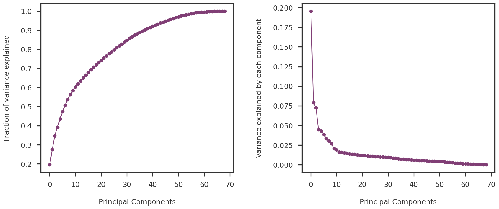
The variance explained by each principal component is shown in Figure 1

fig = plt.figure(figsize = (14, 6))
ax1 = fig.add_subplot(121)
ax2 = fig.add_subplot(122)

#ax1.scatter(np.arange(ncomp), pca.explained_variance_ratio_, s = 100, alpha = 0.7)
ax1.plot(np.arange(ncomp), np.cumsum(pca.explained_variance_ratio_), marker = 'o')
ax1.set_ylabel("Fraction of variance explained")
ax1.set_xlabel("Principal Components")

ax2.plot(np.arange(ncomp), pca.explained_variance_ratio_, marker = 'o')
ax2.set_ylabel("Variance explained by each component")
ax2.set_xlabel("Principal Components")

plt.tight_layout(w_pad = 3)
plt.show()

Figure 1: Variance explained by the Principal Components

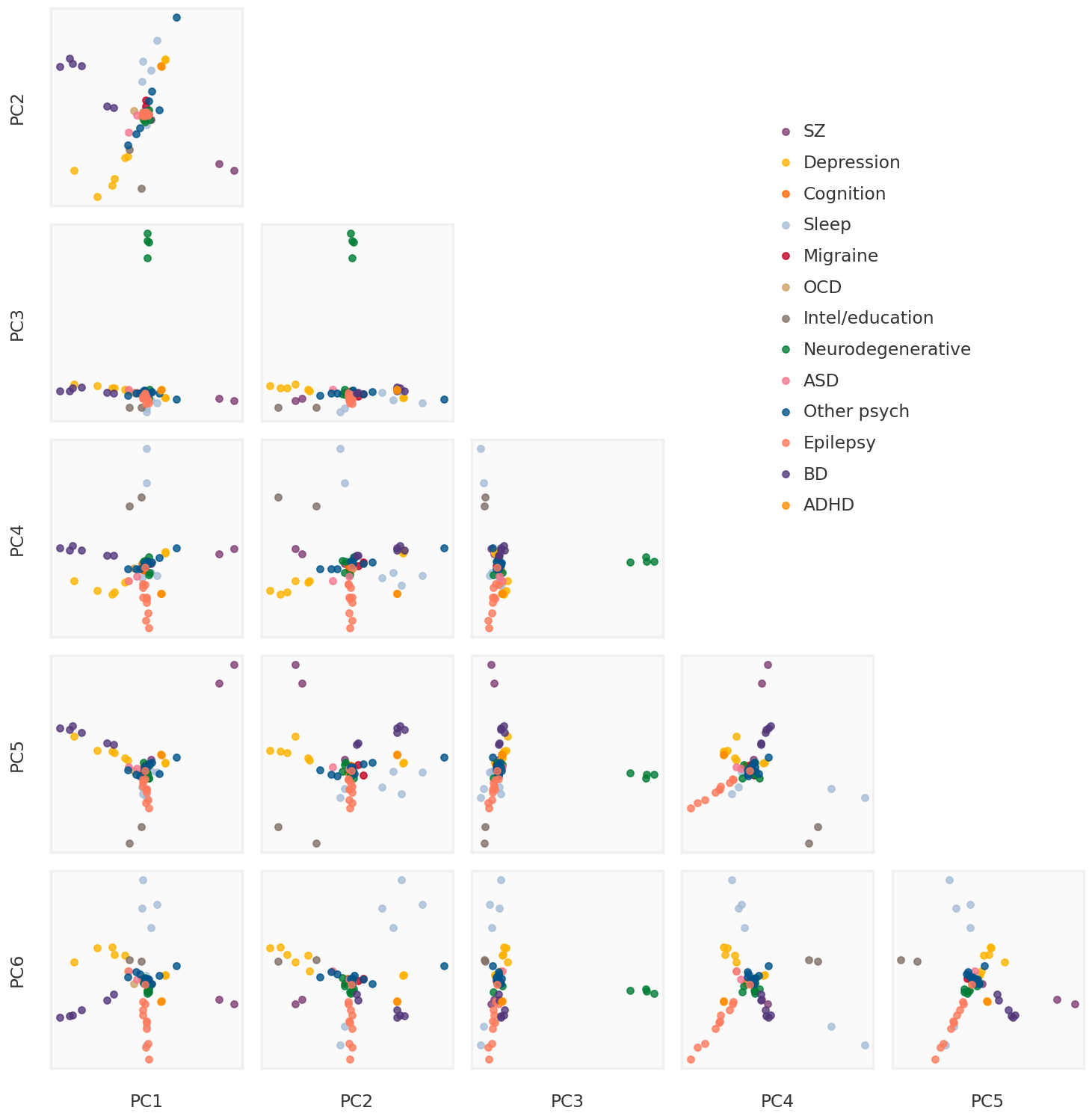
We plot the first 6 principal components against each other in Figure 2. Each dot is a sample (phenotype) colored by their broad label of NPD.

plot_ncomp = 6
subplot_h = 2.0

nrow = plot_ncomp - 1
ncol = plot_ncomp - 1
figw = ncol * subplot_h + (ncol - 1) * 0.3 + 1.2
figh = nrow * subplot_h + (nrow - 1) * 0.3 + 1.5
bgcolor = '#F0F0F0'


def make_plot_principal_components(ax, i, j, comp):
    pc1 = comp[:, j]
    pc2 = comp[:, i]
    for label in unique_labels:
        idx = np.array([k for k, x in enumerate(labels) if x == label])
        ax.scatter(pc1[idx], pc2[idx], s = 30, alpha = 0.8, label = label)
    return

fig = plt.figure(figsize = (figw, figh))
axmain = fig.add_subplot(111)

for i in range(1, nrow + 1):
    for j in range(ncol):
        ax = fig.add_subplot(nrow, ncol, ((i - 1) * ncol) + j + 1)
        
        ax.tick_params(bottom = False, top = False, left = False, right = False,
                       labelbottom = False, labeltop = False, labelleft = False, labelright = False)
        if j == 0: ax.set_ylabel(f"PC{i + 1}")
        if i == nrow: ax.set_xlabel(f"PC{j + 1}")
        if i > j:
            ax.patch.set_facecolor(bgcolor)
            ax.patch.set_alpha(0.3)
            make_plot_principal_components(ax, i, j, beta_pcs)
            for side, border in ax.spines.items():
                border.set_color(bgcolor)
        else:
            ax.patch.set_alpha(0.)
            for side, border in ax.spines.items():
                border.set_visible(False)
                
        if i == 1 and j == 0:
            mhandles, mlabels = ax.get_legend_handles_labels()

axmain.tick_params(bottom = False, top = False, left = False, right = False,
                   labelbottom = False, labeltop = False, labelleft = False, labelright = False)
for side, border in axmain.spines.items():
    border.set_visible(False)
axmain.legend(handles = mhandles, labels = mlabels, loc = 'upper right', bbox_to_anchor = (0.9, 0.9))
          
        
plt.tight_layout()
plt.show()

Figure 2: First 6 principal components compared against each other.

PCA using SVD

Just to make sure that I understand things correctly, I am redoing the PCA using SVD. It must yield the same results as sklearn PCA. Indeed, it does as shown in Figure 3.

U, S, Vt = np.linalg.svd(Xcent, full_matrices=False)
svd_pcs = U @ np.diag(S)

idx1 = 0
idx2 = 1
svd_pc1 = svd_pcs[:, idx1]
svd_pc2 = svd_pcs[:, idx2]

fig = plt.figure()
ax1 = fig.add_subplot(111)

for label in unique_labels:
    idx = np.array([i for i, x in enumerate(labels) if x == label])
    ax1.scatter(svd_pc1[idx], svd_pc2[idx], s = 100, alpha = 0.7, label = label)
    
# idxs = np.array([i for i, x in enumerate(labels) if x == 'Sleep'])
# for idx in idxs:
#     pid = select_ids[idx]
#     ax1.annotate(pid, (svd_pc1[idx], svd_pc2[idx]))

    
ax1.legend(bbox_to_anchor=(1.04, 1), loc="upper left")
ax1.set_xlabel(f"Component {idx1}")
ax1.set_ylabel(f"Component {idx2}")
plt.show()

Figure 3: Check PCA using SVD.

Weighted PCA

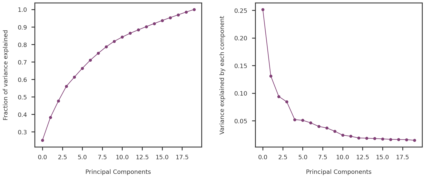
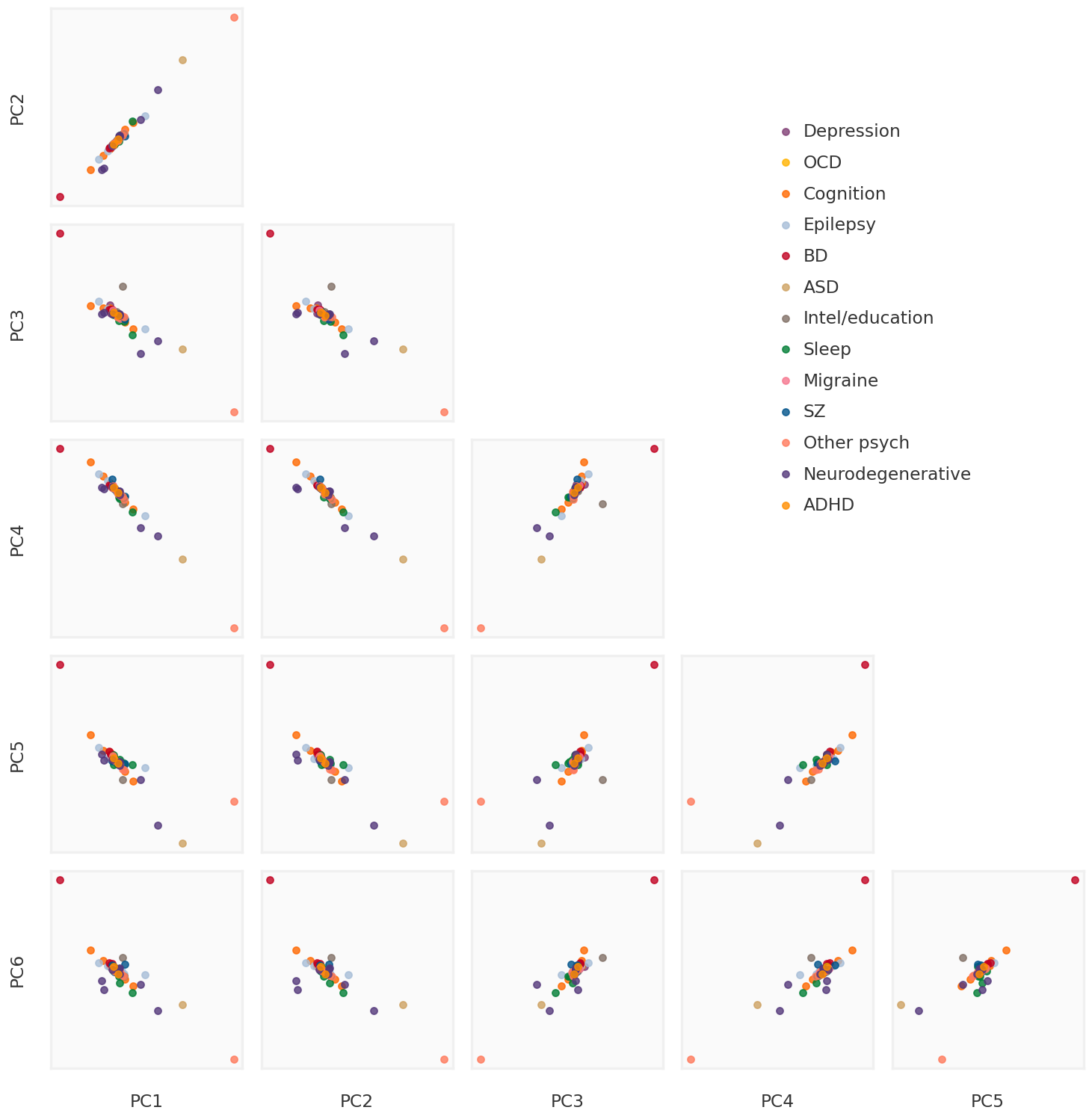
Here, I implement the weighted covariance eigendecomposition approach algorithm proposed by L. Delchambre (2014). I used 3 different versions of the weight matrix:

• the identity matrix (to check that the implementation is correct).
• the precision matrix (as suggested by David in the project proposal).
• square root of the precision (ad-hoc idea to reduce the weights on each observation)

# W = np.ones(X.shape)
# W = np.array(prec_df[select_ids]).T
W = np.sqrt(np.array(prec_df.replace(np.nan, 0)[select_ids]).T)

def weighted_mean(x, w=None, axis=None):
    """Compute the weighted mean along the given axis

    The result is equivalent to (x * w).sum(axis) / w.sum(axis),
    but large temporary arrays are not created.

    Parameters
    ----------
    x : array_like
        data for which mean is computed
    w : array_like (optional)
        weights corresponding to each data point. If supplied, it must be the
        same shape as x
    axis : int or None (optional)
        axis along which mean should be computed

    Returns
    -------
    mean : np.ndarray
        array representing the weighted mean along the given axis
    """
    if w is None:
        return np.mean(x, axis)

    x = np.asarray(x)
    w = np.asarray(w)

    if x.shape != w.shape:
        raise NotImplementedError("Broadcasting is not implemented: "
                                  "x and w must be the same shape.")

    if axis is None:
        wx_sum = np.einsum('i,i', np.ravel(x), np.ravel(w))
    else:
        try:
            axis = tuple(axis)
        except TypeError:
            axis = (axis,)

        if len(axis) != len(set(axis)):
            raise ValueError("duplicate value in 'axis'")

        trans = sorted(set(range(x.ndim)).difference(axis)) + list(axis)
        operand = "...{0},...{0}".format(''.join(chr(ord('i') + i)
                                                 for i in range(len(axis))))
        wx_sum = np.einsum(operand,
                           np.transpose(x, trans),
                           np.transpose(w, trans))

    return wx_sum / np.sum(w, axis)

def weighted_pca_delchambre(X, W, n_components = None, regularization = None):
    
    import scipy as sp
    
    weights = weighted_mean(X, W, axis = 0).reshape(1, -1)
    _X = (X - weights) *  weights
    _covar = np.dot(_X.T, _X)
    _covar /= np.dot(weights.T, weights)
    _covar[np.isnan(_covar)] = 0

    n_components = 20
    eigvals = (_X.shape[1] - n_components, _X.shape[1] - 1)
    evals, evecs = sp.linalg.eigh(_covar, subset_by_index = eigvals)

    components = evecs[:, ::-1].T
    explained_variance = evals[::-1]
    Y = np.zeros((_X.shape[0], components.shape[0]))
    for i in range(_X.shape[0]):
        cW = components * weights[0, i]
        cWX = np.dot(cW, _X[i])
        cWc = np.dot(cW, cW.T)
        if regularization is not None:
            cWc += np.diag(regularization / explained_variance)
        Y[i] = np.linalg.solve(cWc, cWX)
    return Y, explained_variance

weighted_pcs, explained_variance = weighted_pca_delchambre(Xcent, W, n_components = 20, regularization = None)

As before, the variance explained by each principal component is shown in Figure 4

wpca_tot_explained_variance = np.sum(explained_variance)
wpca_explained_variance_ratio = explained_variance / wpca_tot_explained_variance

fig = plt.figure(figsize = (14, 6))
ax1 = fig.add_subplot(121)
ax2 = fig.add_subplot(122)

ax1.plot(np.arange(20), np.cumsum(wpca_explained_variance_ratio), marker = 'o')
ax1.set_ylabel("Fraction of variance explained")
ax1.set_xlabel("Principal Components")

ax2.plot(np.arange(20), wpca_explained_variance_ratio, marker = 'o')
ax2.set_ylabel("Variance explained by each component")
ax2.set_xlabel("Principal Components")

plt.tight_layout(w_pad = 3)
plt.show()

Figure 4: Variance explained by the weighted Principal Components

We plot the first 6 principal components against each other in Figure 5. Each dot is a sample (phenotype) colored by their broad label of NPD.

plot_ncomp = 6
subplot_h = 2.0

nrow = plot_ncomp - 1
ncol = plot_ncomp - 1
figw = ncol * subplot_h + (ncol - 1) * 0.3 + 1.2
figh = nrow * subplot_h + (nrow - 1) * 0.3 + 1.5
bgcolor = '#F0F0F0'


def make_plot_principal_components(ax, i, j, comp):
    pc1 = comp[:, j]
    pc2 = comp[:, i]
    for label in unique_labels:
        idx = np.array([k for k, x in enumerate(labels) if x == label])
        ax.scatter(pc1[idx], pc2[idx], s = 30, alpha = 0.8, label = label)
    return

fig = plt.figure(figsize = (figw, figh))
axmain = fig.add_subplot(111)

for i in range(1, nrow + 1):
    for j in range(ncol):
        ax = fig.add_subplot(nrow, ncol, ((i - 1) * ncol) + j + 1)
        
        ax.tick_params(bottom = False, top = False, left = False, right = False,
                       labelbottom = False, labeltop = False, labelleft = False, labelright = False)
        if j == 0: ax.set_ylabel(f"PC{i + 1}")
        if i == nrow: ax.set_xlabel(f"PC{j + 1}")
        if i > j:
            ax.patch.set_facecolor(bgcolor)
            ax.patch.set_alpha(0.3)
            make_plot_principal_components(ax, i, j, weighted_pcs)
            for side, border in ax.spines.items():
                border.set_color(bgcolor)
        else:
            ax.patch.set_alpha(0.)
            for side, border in ax.spines.items():
                border.set_visible(False)
                
        if i == 1 and j == 0:
            mhandles, mlabels = ax.get_legend_handles_labels()

axmain.tick_params(bottom = False, top = False, left = False, right = False,
                   labelbottom = False, labeltop = False, labelleft = False, labelright = False)
for side, border in axmain.spines.items():
    border.set_visible(False)
axmain.legend(handles = mhandles, labels = mlabels, loc = 'upper right', bbox_to_anchor = (0.9, 0.9))
          
        
plt.tight_layout()
plt.show()

Figure 5: First 6 weighted principal components compared against each other.

Further Reading

• Comments on PCA by Alex Williams